


In Part 1, we argued that LLM routing is qualitatively different from HTTP routing. Inference backends hold state that traditional load balancers ignore. This post covers the first of the three layers we identified: the data layer that makes that state queryable on the hot path of every inference request.
To route a request to the pod with the best cached prefix, you need to know which blocks are cached on which pod. That sounds simple until you look at the numbers. You may have hundreds of pods, each with thousands of cached blocks. State can change hundreds of times per second. Across this complexity, queries need to return in microseconds because they sit on the critical path of every inference request.
A hashmap and a mutex aren’t sufficient for the scale and velocity of inference routing. You need a data structure designed for this specific access pattern: a way to provide fast concurrent reads, batched writes, idempotent event processing, and efficient query responses.
This post walks through how we built that data structure.
The problem
Given a request tokenized into N block hashes (the query chain) and P live pods in the cluster, return a ranked list of pods ordered by how many of those N blocks each pod has cached.
The constraints:
- Microsecond-level query latency. This runs on the hot path and every inference request goes through it.
- Concurrent with ongoing updates. Pods are constantly caching and evicting blocks. Queries and updates happen simultaneously.
- Resilient to pod churn. Pods are added and removed as deployments scale or restart. The index needs to reflect the current live set without stale entries accumulating over time.
- Accurate enough to route correctly. Not perfectly consistent (some staleness is fine) but accurate enough that the pod we pick actually has the cache we expect.
For a concrete example: say we have 64 pods, 32 blocks per query, 1,000 requests per second. A naive approach (for each block, for each pod, check if the pod has it cached) is 32 × 64 = 2,048 lookups per request. That’s over 2 million per second in aggregate. Lock contention aside, this approach cannot meet the microsecond latency constraint. We need something different.
Where state comes from
The data layer doesn't originate cache state. It consumes it.
LLM engines emit block-level events as their cache contents change:
- Registered: a block has been cached in a particular memory tier on a particular pod.
- Evicted: a block has been removed from a tier on a pod.
- Shutdown: a pod is going away.
How those events reach the routing layer depends on the deployment. Some environments use a pub/sub fabric like NATS with JetStream. Others use direct gRPC streams from each engine instance to the router. Future deployments might use Kafka, Redis Streams, or something else entirely.

The data layer's job is to be indifferent to the transport. Adding a new event source means implementing one consumer interface. The indexer sees a stream of typed events and doesn't know or care what message infrastructure they came from.
Two requirements follow from this design.
Idempotent operations. The same event might arrive twice. A replay of the last hour of block events on a consumer restart is normal. Registering a block that's already indexed is a no-op. Evicting a block that's already gone is a no-op. Shutting down a pod that's already dead is a no-op. These are valid states, not error cases.
Multi-consumer safety. Two consumers (for example NATS and gRPC) might feed the same indexer simultaneously. They shouldn't conflict. This is guaranteed by idempotency: if both consumers see "pod A registered block X" and both write it, the result is the same as one consumer writing it once.
Storage: the HostBitmap
The central question the index answers is: which pods have this block?
The naive representation is a slice of pod identifiers per block: blockHash → [podA, podC, podF]. It works, but it's wasteful in ways that compound at scale. Every pod identifier is a string pointer. Every slice has its own backing array and header. Millions of small heap allocations put sustained pressure on Go's garbage collector. And checking "does pod X have block Y?" means a linear scan over the slice.
The question is a set-membership test across a bounded population of pods, which is most efficiently represented as a bitmap.
A bitmap assigns each pod an index (0, 1, …, P−1) and represents "the set of pods that have this block" as a fixed-width bit vector. One bit per pod. Set operations (union, intersection, complement) become bitwise operations. Membership is a single bit test. Population count compiles down to a single POPCNT instruction on x86-64.
We cap pod count at 256 as a deployment-level design choice. 256 is larger than any single-orchestrator deployment we've seen in production and it could be widened in the future without requiring a redesign. At 256 pods, the bitmap is 256 bits = 32 bytes = four uint64 words. The HostBitmap type is four uint64s laid out flat. We cap the pod count per orchestrator instance. This fits naturally with a cell-based deployment architecture, where each routing instance owns a self-contained cell of pods and horizontal scale comes from running more cells rather than widening any one. The cap is larger than any single-cell deployment we have seen in production, and we could widen it later without redesigning the data structure. The HostBitmap is a fixed-size flat array of uint64 words sized to the cap, with no pointers, heap allocation, or indirection.

The full index is map[blockHash] → HostBitmap. For every block the cluster has cached anywhere, the map stores which pods have it.
Concurrency: sharding the index
A single map[blockHash] → HostBitmap works until concurrent writes go behind a lock. Then every update (every Registered or Evicted event) serializes against every other update and every read. At hundreds of events per second across thousands of blocks, the lock becomes the bottleneck.
The fix is sharding. We split the index into 256 independent maps, each with its own lock. A block’s shard is chosen by hashing the block hash and taking the top bits. We picked 256 because it makes per-shard contention negligible at our target throughput while keeping memory overhead trivial. Writes to different shards proceed in parallel, as do reads. Reads and writes to the same shard still contend, but only for a single map operation, not a full scan.
Fibonacci hashing for shard distribution
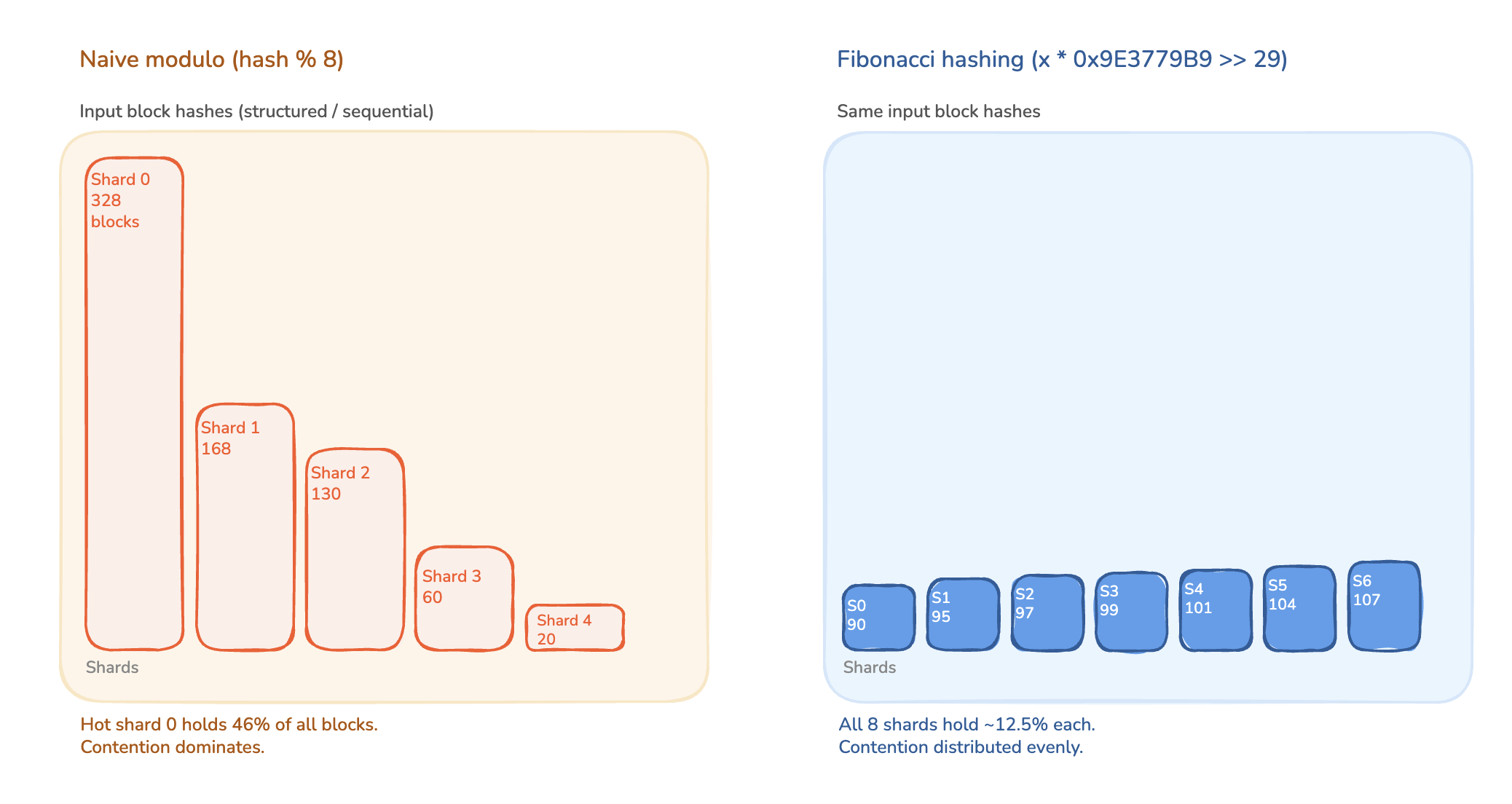
Block hashes from cumulative hashing aren't uniformly random. They carry structure that reflects the input token distribution. Using the low bits of the hash directly for shard selection would cluster related blocks into the same shard, turning 256-way parallelism back into a handful of hot shards.
We run the block hash through a multiplicative hash with the golden-ratio constant (0x9E3779B97F4A7C15 for 64-bit), a technique known as Fibonacci hashing, before extracting the shard index from the top bits. The golden-ratio multiplier is 2^64 divided by φ (the golden ratio, ≈ 1.618). Even sequential inputs scatter across the output range with maximum spacing between consecutive images, a result that follows from the three-distance theorem.
Cache-line padding
Each shard struct is padded so it starts on its own 64-byte cache-line boundary. Without padding, two adjacent shards might share a cache line. A write to one invalidates the line on every CPU core that has the other cached. This is false sharing and it quietly kills concurrency on workloads that look parallelism-friendly. The padding costs ~16 KB total (256 shards × 64 bytes) and eliminates the problem entirely.
With 256 shards and Fibonacci distribution, the probability that any given block lands in a specific shard is 1/256. At 1,000 QPS (queries per second) with 32 blocks per query, each shard sees roughly 125 lookups and a handful of writes per second. Contention is effectively minimized.
Query: prefix matching with binary search
Storage handles "does pod X have block Y?" in constant time. Routing needs to answer a harder question: for a query chain of N blocks, how many of them does each pod have?
The naive approach is the N x P loop. For each of the N blocks in the query chain, look up the bitmap in its shard, then check each of the P pods. At 64 pods and 32 blocks, that's 2,048 shard lookups per request. At 1,000 QPS this would require over 2 million lookups per second, making it impossible to meet the microsecond query latency target.
Cumulative block hashing is the solution. Block hashes in our system aren't independent. Each block's hash is a function of its own tokens and the hash of the previous block. Block 4's hash incorporates everything from blocks 0 through 3.
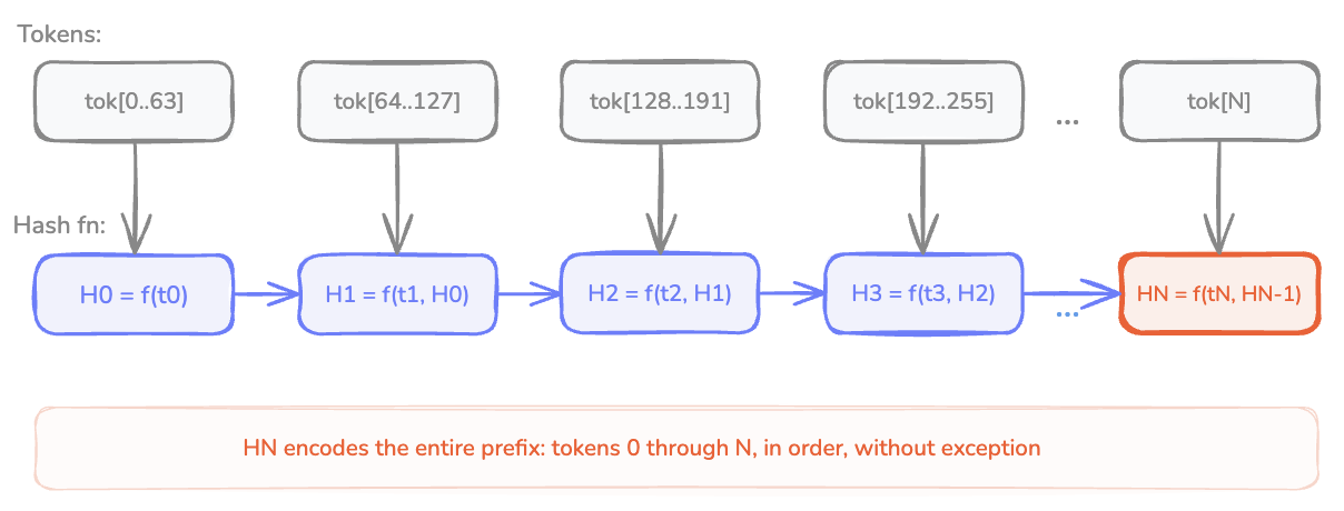
The consequence: if a pod has block 5 cached with a particular hash, it must have computed blocks 0 through 4 with exactly the same chain of hashes. Cache hits form a contiguous prefix. There's no "I have block 5 but not block 3." If the block-5 hash matches, the prefix up to block 4 matched too.
This turns the query from a N x P scan into a binary search for the drop-off point: the largest K such that each pod has the first K blocks of the query chain cached. Because the prefix is contiguous, binary search applies.
Worked example
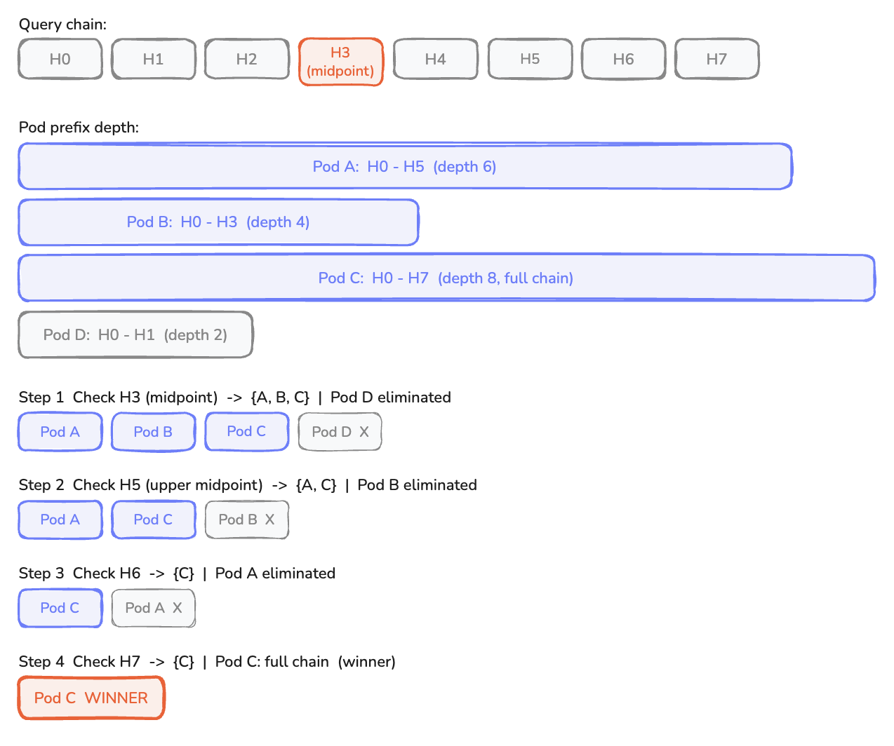
Here’s an example of binary search prefix matching using four pods and eight blocks.
Step 1. Check block H3 (midpoint). Look up the shard for H3, intersect the bitmap with the alive-pods bitmap.
Result: {A, B, C}. Pod D dropped off before H3.
Step 2. For the survivors {A, B, C}, check H5 (midpoint of upper half).
Result: {A, C}. Pod B dropped off between H3 and H5.
Step 3. Check H6.
Result: {C}. Pod A dropped off between H5 and H6.
Step 4. Check H7.
Result: {C}. Pod C has the full chain.
For pods that dropped off (A, B, D), we binary-search their exact drop-off depths. Total shard lookups in this example: roughly 10. The naive P × N scan would take 32.
Time complexity
The complexity is O(K × log N), where K is the number of distinct drop-off depths across the surviving pod set. If all pods have the same prefix depth, K = 1 and the search finishes in log N lookups. If every pod has a different depth, K = P.
In practice, pods in the same deployment tend to have similar cache states (they've all handled prior requests from the same distribution) so K is small.
The binary search cost scales with log N and K, neither of which is large. It does not scale with P. Doubling the pod count doesn't change the number of shard lookups. It changes the population count on the bitmaps, which is a constant-time operation per word.
Correctness: chaining and availability are different
Two different problems in this data layer both involve hashing, and it's worth being precise about what each one solves.
Cumulative chaining solves a correctness problem. Two different requests might happen to share the same tokens in block 3 while differing earlier in the sequence. If blocks were identified only by a local hash of their own tokens, those requests would produce the same H3 and the router would treat their block-3 KV cache entries as interchangeable. They aren't: the attention values depend on the full context, not just the local tokens. Sharing cache across mismatched prefixes produces incorrect model output.
Cumulative chaining ensures that every block hash encodes the full token sequence up to that point, not just the tokens in that block. Two requests that happen to share the same tokens in block 3 but differ earlier in the sequence will produce different H3 values. The KV cache entries are distinct, so the router treats them as distinct — and the model sees the right context.
Bitmap lookup solves an availability problem. Given a hash chain that's correct, which of those hashes is actually present on which pods right now? Blocks get evicted. Pods crash. The hash chain describes what a pod's cache would need to contain to serve a request; the bitmap records what it actually contains. Routing needs both: chaining to ask the right question, and bitmaps to answer it accurately against live cluster state.
Tiered storage: where the block lives
As deployments add CPU-memory and SSD offload tiers (covered in our Five Eras of KV Cache post), the question expands from "does this pod have the block?" to "where on this pod does it live?" GPU memory is strictly faster than CPU memory, which is strictly faster than SSD. The router should prefer pods that have the block in the fastest accessible tier.
The tempting approach is to extend the HostBitmap to be per-tier: three bitmaps per block instead of one. That works, but it bloats the hot path. Most routing decisions don't need per-tier information. They just need "who has this block?" Paying the extra cost on every query is wasteful.
Instead, we split the index into two layers.
Routing shards. The 256-shard HostBitmap index described above. Answers "who has this block?" on the hot path. This is queried on every request.
Host tier maps. A separate per-pod data structure that answers "where on this pod does this block live?" The tier map is consulted only after a winning pod is selected, to produce the cache hint injected into the downstream request.

The split follows naturally from the access pattern. Routing decisions query the hot path on every request. Tier information is pulled only for the winner. The two data structures can be sized and tuned independently.
Host lifecycle: two-phase removal
Pods come and go. When a pod's events stop arriving (whether it crashed, was evicted, or is draining) the indexer needs to stop routing to it immediately. When a new pod takes its slot, routing needs to pick it up.
The naive approach is to walk every shard and clear the dead pod's bit from every bitmap. For tens of thousands of blocks, this holds shard locks for a long time and blocks routing queries.
We use two-phase removal instead.
Phase 1: instant liveness update. Every pod has a bit in a global alive bitmap, separate from the per-block shards. When a pod is declared dead, we compare-and-swap (CAS) its bit to 0 in the alive bitmap. Every subsequent routing query intersects candidate bitmaps with the alive bitmap, so the dead pod is instantly excluded without touching a single shard.
Phase 2: bounded concurrency cleanup. The per-block shard entries for the dead pod are still there, masked out by the alive bitmap. A background goroutine walks the shards with a bounded concurrency limit and clears the dead pod's bits. When cleanup finishes, two things are reclaimed: the dead pod's per-tier maps of block → location (offset, length, device), and routing-shard entries for blocks that the dead pod was the last live holder of. Without this second sweep, block hashes that no surviving pod holds would accumulate in the index as the cluster churns. The result of these phases is that hot path stays fast. Cleanup happens at the indexer's own pace without blocking routing.
Putting it together
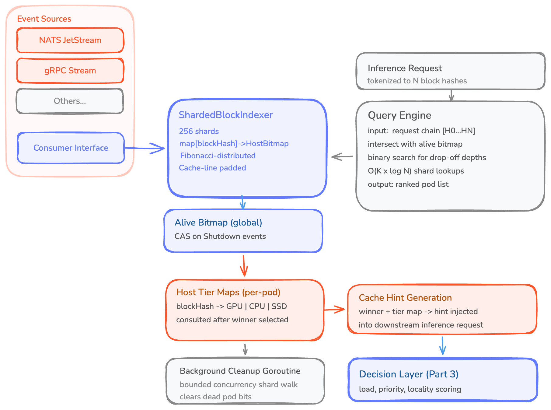
The data layer in Modular Cloud's routing system:
- A ShardedBlockIndexer with 256 shards. Each shard maps blockHash → HostBitmap. Fibonacci-distributed so related blocks scatter. Cache-line-padded to avoid false sharing.
- A separate alive bitmap for pod liveness, CAS-updated on shutdown events.
- Per-pod tier maps for the cold path that resolves winning candidates to cache-hint locations (GPU/CPU/SSD).
- Event consumers (NATS, gRPC, others) that push Registered/Evicted/Shutdown events into the indexer through idempotent operations. Transport-agnostic by design.
- A query path that answers "how many blocks from this chain does each pod have?" via binary search over the cumulative hash chain: O(K × log N) shard lookups instead of P × N.
The result is a data structure that handles tens of thousands of queries per second on the hot path of an inference orchestrator while concurrent event streams update it in real time.
Conclusion
Cache-aware routing is only as fast as the data layer underneath it. If answering "which pods have these blocks?" takes milliseconds, you've spent the latency budget before any scoring logic runs. The architecture here (sharded bitmaps, Fibonacci-distributed for uniformity, queried via binary search over cumulative block hashes, with two-phase host lifecycle for pod churn) keeps that answer in the microsecond range.
The data layer answers one question: who has the cache? Cache affinity is one input into a routing decision. Load, session state, tenant priority, hardware role, node locality for KV cache transfer: these all come into play, and different deployments weight them differently. The data layer gives you the facts. The decision layer tells you what to do with them.
What's next
Part 3 covers the decision and execution layers: turning cache state into routing decisions, then into execution. A five-stage composable pipeline, typed state between plugins, and the Selector/Workflow/Executor split that scales the same framework from round-robin to disaggregated prefill/decode.