


🛠️ Code to all kernels mentioned in this series is available on GitHub.
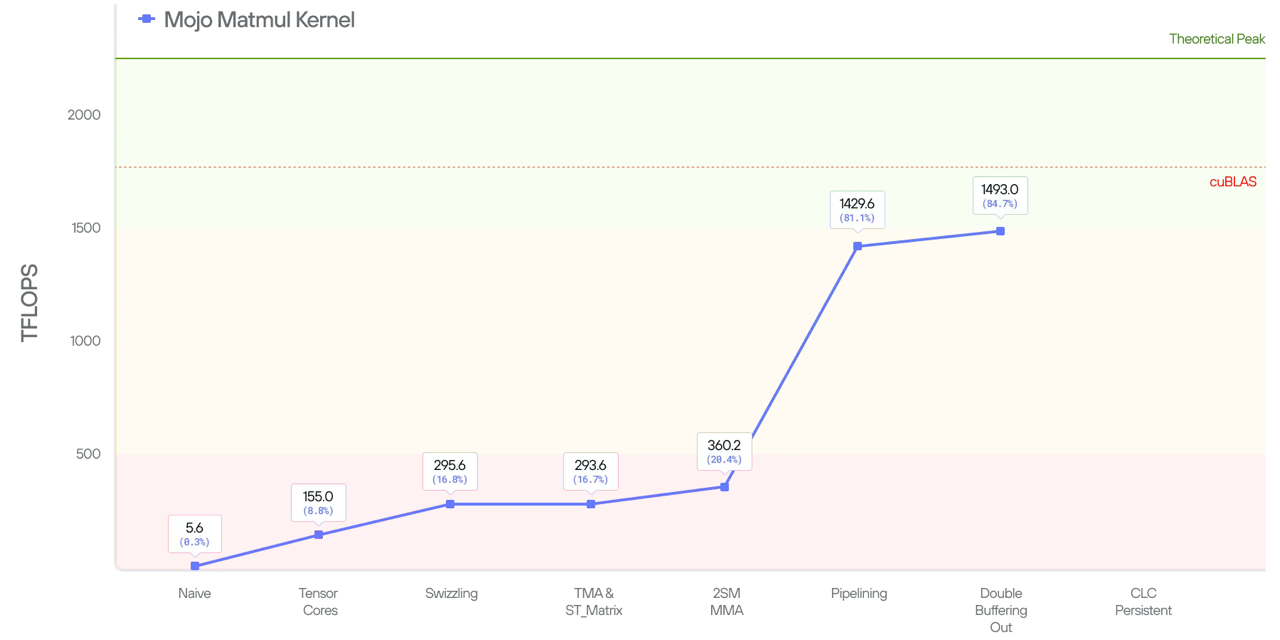
In the prior blog posts in this series (part 1 and part 2) we talked about how to achieve ~300GFlops performance for Matmul on NVIDIA Blackwell GPUs. In this post, we continue on this journey and discuss how to leverage the 2SM technique along with pipelining to increase our performance about 5x and get within 85% of state-of-the-art (SOTA).
Kernel 5: multicast and 2xSM MMA
Since NVIDIA’s Hopper generation, Streaming Multiprocessors (SMs) can be grouped, and Cooperative Thread Arrays (CTAs) within the same SM group can access each other’s shared memory (also known as distributed shared memory access). This brings up two advanced optimizations on Blackwell:
- Tensor Memory Accelerator (TMA) multicasting—supported since Hopper: SMs collaborate on loading a tile into shared memory.
- 2xSM Matrix Multiply-Accumulate (MMA): 2 SM's tensor cores collaborate on one large MMA operation using inputs in SM's shared memory.
Let’s examine both techniques and see how they are reflected in code. The first thing we need to do is inform the code about the size of the cluster (the cluster_shape). Find the code for Kernel 5 here. This can be done in Mojo using the @__llvm_metadata decorator:
The above sets the “CTA cluster” launch shape for the kernel at compile time. CTAs within in the same cluster can access to each others’ shared memory.
CTA memory multicasting
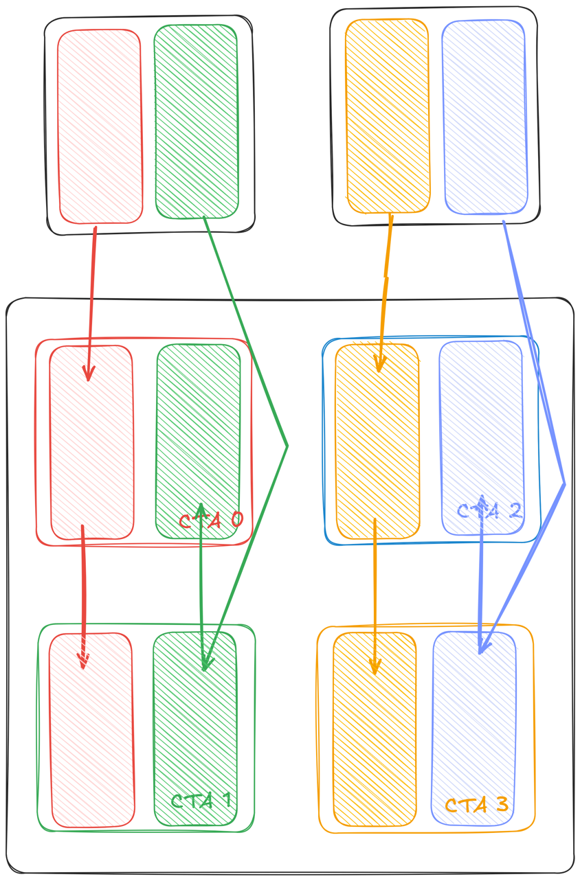
To understand memory multicasting, let’s take a simple example and examine what we’d have to do without the multicasting feature. For visualization, we will use A, B, and C as 256x256 matrices. In this case, we will launch 4 CTA’s.
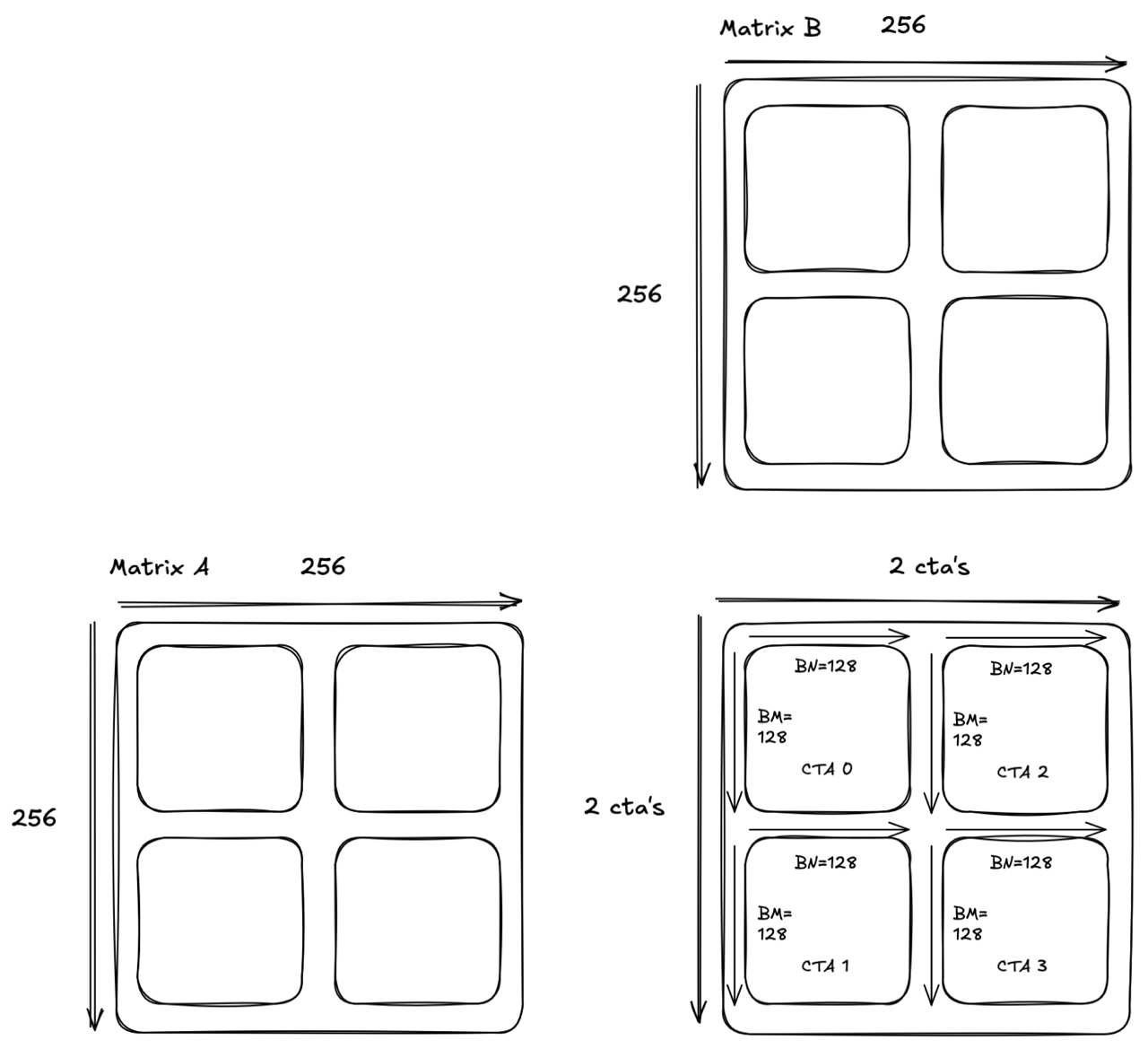
Each CTA will compute a 128x128 tile. Let’s examine which tiles CTA each loads throughout K/BK:
Note the redundancy in the memory loads. This is similar to the redundancy we noticed at the beginning of the blog series, but this time the redundancy is occurring at tile granularity instead of element granularity.
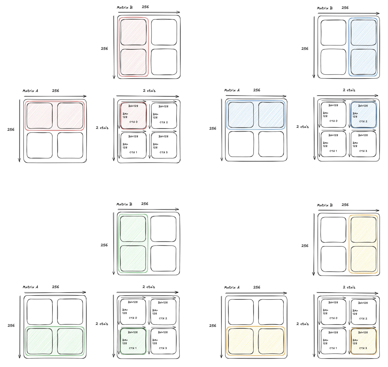
How can we mitigate this? If we group these 4 CTAs into a 2x2 cluster, the SMs can now access each others’ shared memory, which allows each SM to load a tile from global memory and then broadcast the memory to its neighbors.
With this capability, we can adjust our load strategy and have the two CTA’s along the same row load exactly one half of the tile from A, and to broadcast that half to their neighbor. That way, both CTA’s do half the loads while still getting the full tile. Visually, this looks like:
We can extend this technique to save the loads for the B matrix as well:
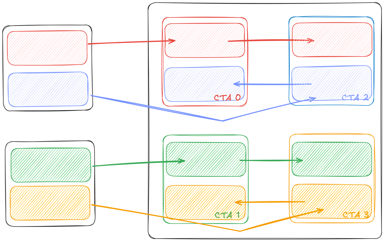
This technique is called multicasting and is scalable. For example, when launching a 4x4 cluster we’d make each CTA load half of its tiles and get the rest of the data from its peers. Let’s look at how this is implemented in Mojo. We begin by declaring the TMA ops on the host side:
Since each CTA will slice the shared memory tiles for A and B and broadcast them to corresponding peer CTAs, we divide the TMA tile by the cluster dimension. In the GPU kernel, we launch the multicast load using:
The API is similar to the async_load TMA API we showed in our last blog but with a few key differences, discussed in the following paragraphs.
First, there is an additional TMA mask a_multicast_mask. The TMA mask is a 16 bit value describing the CTA index involved in the load. Each bit stands for one CTA and there can be at most 16 CTAs in one cluster. For example, in the above CTA 0 and 2 multicast the A tile so the CTA masks are both 0b101. In Mojo we can compute that via:
The layout tensor a_smem_slice is sliced from the original tile by offsetting the base pointer:
We also update the corresponding coordinates in global memory for this tile slice:
2xSM MMA
We have shown how distributed shared memory and multicast can help reduce the data volume from global memory to shared memory. However there is still one limitation—the tiles are duplicated in the distributed shared memory. Looking into CTAs 0 and 1 in the previous example, we see both CTAs keep a copy of BNxBK tile in shared memory, as shown in the left side of Figure 6 below. Given each CTA has access to the other’s shared memory, saving two copies of the same tile is a waste of resources.
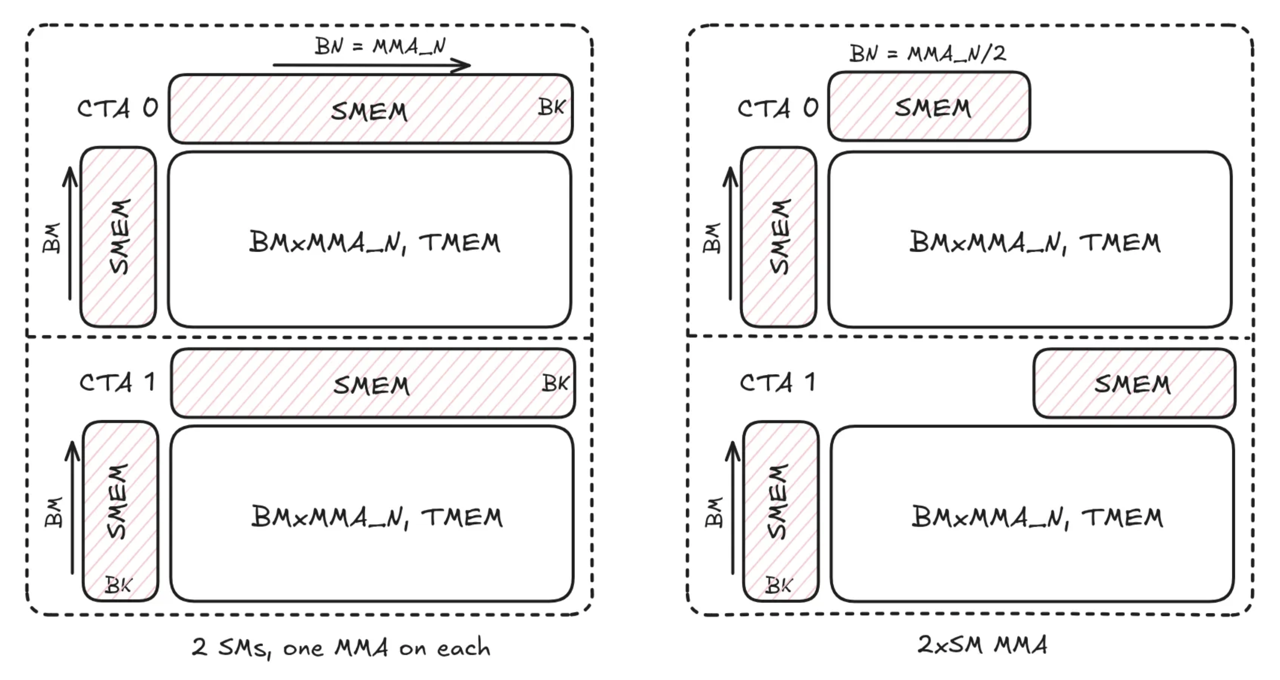
Blackwell’s 2xSM MMA instruction (tcgen05.mma.cta_group::2) is designed to address this problem. As shown in the right side of Figure 6, CTAs 0 and 1 works as a pair and each only loads half of the B tile. The 2xSM MMA instruction sees both halves in shared memory and coordinates the tensor cores on both SMs to complete MMA operations as large as two single SM MMAs. Comparing the left and right figures above, the 2 SMs are calculating the same MMA workload 2*BM x MMA_N x BK , where MMA_N denotes the N dimension of MMA shape, and producing the same result, however the 2xSM instruction reduces the shared memory usage for the B tile by half.
Comparing to multicast load with single SM MMA, the 2xSM MMA load reduces shared memory traffic in two ways. First, CTAs 0 and 1 still load the same half of the B tile as in multicast load (see Figure 5) but it’s only a regular TMA transfer, i.e. the multicast step is omitted. Moreover, the traffic from shared memory to tensor memory for the B tile is also halved as we only save one copy of it in the distributed shared memory.
The code to launch 2xSM MMA is quite similar to launching single SM MMA (see our previous blog), with the exception of using elect_one_cta. Since two SMs collaborate on one MMA operation, only one CTA should launch the instruction and that’s the CTA with even ID in each pair of CTAs. Hence, the elect_one_cta is a predicate to select the launching CTA (also called the leader CTA).
The mma function above will invoke the tcgen05.mma.cta_group::2 instruction when cta_group is 2. We also change the arrive function from mma_arrive (see the previous blog) to mma_arrive_multicast, which takes cta_group and signals the leader CTA’s memory barrier when cta_group=2.
Tensor memory layout
With the 2xSM MMA instruction, the two CTAs partition the M dimension (MMA_M) evenly (BM = MMA_M/2 ) and each has half of the result of shape BM x MMA_N in tensor memory. The instruction supports MMA_M values of 128 and 256. For MMA_M=256, the TMEM layout for each half is the same as single SM MMA as shown in Figure 7 below. The top half is stored in the leader CTA with the lower half in its pair CTA. The output to global memory is the same as in kernel 4 from our last post.

For MMA_M = 128, the layout is different than above. We skip the details here and refer the reader to the code since MMA_M = 128 is less important in production.

With this implementation, we are now at 360.2 TFLOPs and about 20% of our SOTA goal. If we look at the profile, even though we are using the advanced MMA instruction, we’re still limited by global memory throughput because the computation still waits for data transfer to complete. Our next optimization is going to remove this barrier and increase the overlap between computation and memory transfer.
Kernel 6: 2SM pipelining
To keep the code clean throughout the explanation of this kernel, we wrap up the logic we use to load tiles into shared memory through a function call to load_AB(), and we wrap up the logic for calling the MMA through a function call consume_AB(). We further abstract the code to write it out with a function call to store_C. The code for kernel 6 is here.
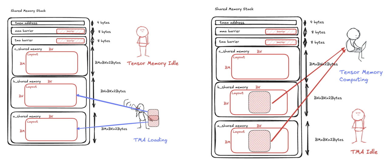
If we operate at this granularity, the previous kernel performs the following:
At any given moment, half of our hardware is idle. Either the tensor cores are waiting for the data to arrive or the TMA is waiting for for MMA to finish so that the shared memory buffer becomes available. The data dependence prevents a CTA from leveraging both hardware units simultaneously.
Pipelining MMA and TMA
The classic algorithm to overcome idleness is to introduce multiple buffers in shared memory and overlap MMA with TMA via pipelining. To exploit this, we need to first check our shared memory usage.
On a Blackwell GPU, the kernel can access up to up to 227 KB shared memory (shared memory and L1 cache combined provide one with 228 KB cache memory, but 1 KB has to be reserved for L1). So far we have the following usage with the largest 2xSM MMA instruction of shape 256x256x16 for BF16:
- one A tile:
BM x BK x 2B = (MMA_M / 2) * 64 * 2B = 16 KB - one B tile:
BN x BK x 2B = (MMA_N / 2) * 64 * 2B = 16 KB - one C tile:
BM x MMA_N x 2B = 64 KB
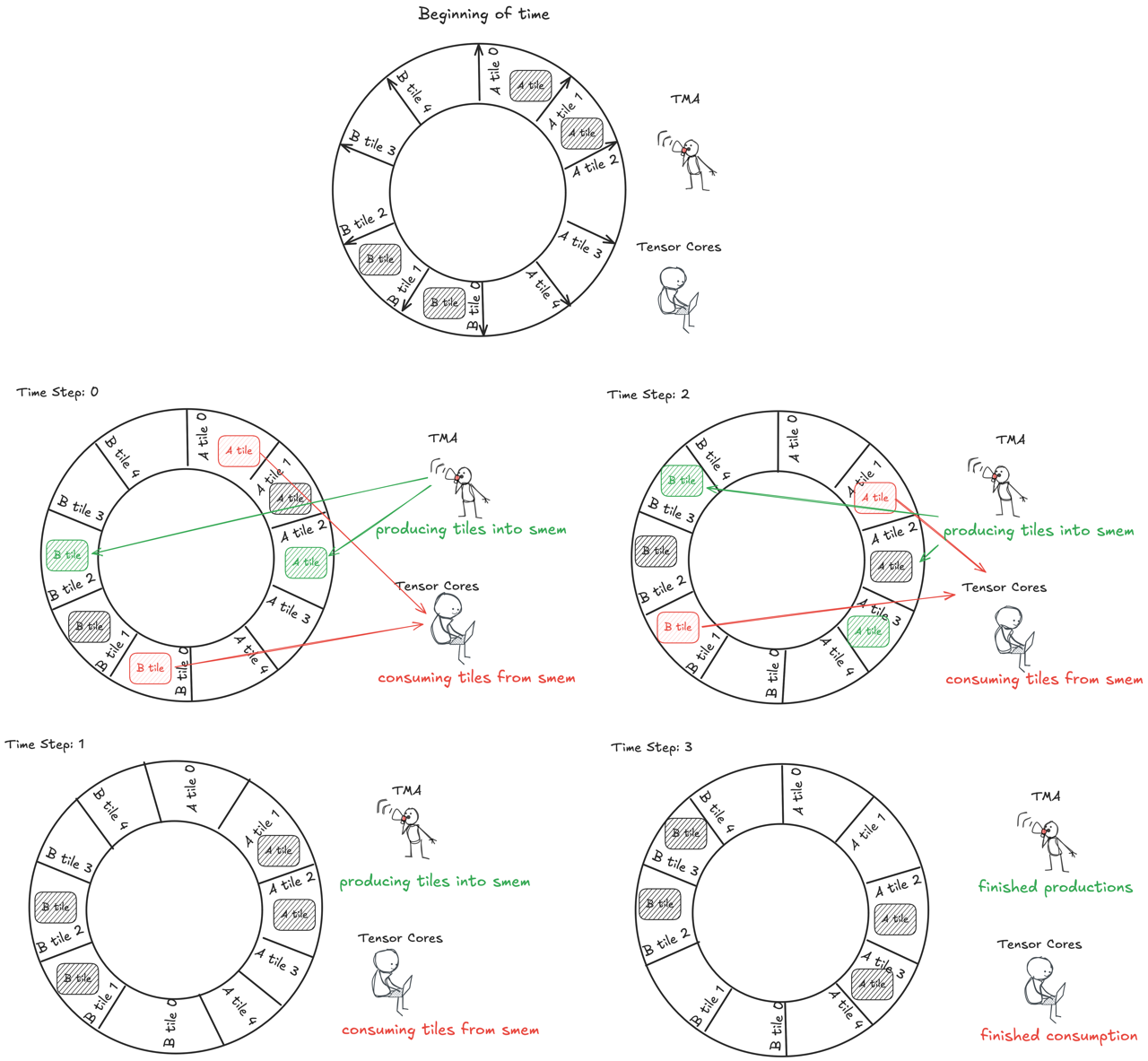
We have used less than half of the capacity. Leveraging the shared memory capacity, we introduce 5 stages and organize them into a circular buffer.

Then we let TMA and MMA iterate through the buffers in parallel such that when MMA is consuming one buffer, another TMA can prefetch data into another buffer for subsequent computation. As a result, we can increase the overlap between computation and communication.
Warp specialization
To implement this pipelined pattern, we need to touch on another important concept—warp specialization. Thus far, we’ve been using 4 warps in previous kernels due to the requirement that loading from TMEM, as well as launching both TMA and MMA, happen in thread 0. To have TMA and MMA issued in parallel and operate on different pipeline stages, we need to specialize different warps for each task. This is called warp specialization. The high level code structure is as follows:
We specialize one warp for issuing TMA and one for issuing MMA and they iterate through the tiles concurrently. Additionally, we need the warps to inform each other if a tile has arrived or has been consumed and the underlying buffer is ready for new data. This communication is done via memory barriers. In the above, we use the same memory barriers as in previous kernels, however the MMA warp waits on the TMA barrier (signaled by the TMA warp) to query if the input is ready for computation. Similarly, the warp specialized for TMA operations waits on MMA barrier to know if buffer is ready for writing new data.
Output
We still need four warps for using TMEM in the output. Following warp specialization, we assign four separate warps for output. In the next post, this will be necessary to overlap output with TMA and MMA. We also need another memory barrier to communicate between MMA and Output warps that the MMA results are ready for output. The high level structure becomes something like:
Here the MMA warp additionally signals a new memory barrier, compute_barrier. Then the output warps waits on compute_barrier to ensure the result is ready. The storing part is same as before.
Benchmarking this pipelining strategy increases our performance and puts us at 1429 TFLOPs, or 81% of SOTA.

Kernel 7: double-buffering the write-out
Thus far we have been optimizing the loading of the data into the matmul, but we can also optimize the storing of the data into the output. First, let’s briefly review how we store the result in TMEM to global memory. The code for kernel 7 is here.
There are three main steps when storing the C data: TMEM to registers, registers to shared memory, and shared memory to global memory. These transfers are executed sequentially due to the data dependence. However, that’s not necessary—especially when TMA store is asynchronous. Applying the same idea as before, we can pipeline the TMA and MMA operations.
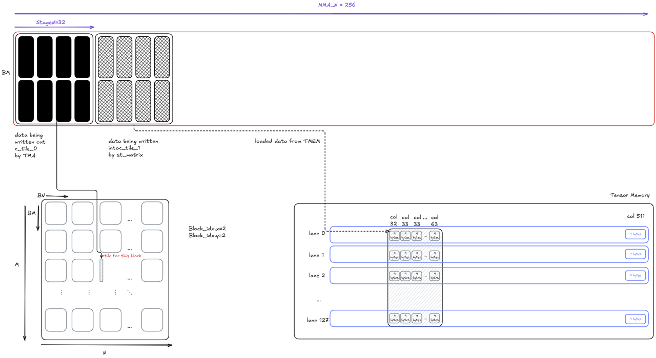
To do that, we declare two output tiles (called the double-buffer) of shape BM x StageN in shared memory and ping-pong between them. For simplicity, we start with stageN = 32 (this is a value that can be tuned). The double-buffer pipeline strategy is illustrated below for two iterations. After stmatrix stores the first output tile to shared memory, we issue the TMA store but don’t block. Instead, we immediately begin loading from TMEM and writing the data into shared memory using the other buffer. Using this scheduling strategy, the TMA store overlaps with the TMEM ⇒ register ⇒ shared memory transfer for the other tile.

To implement the pipeline stategy in Mojo, we first break down the output into MMA_N / StageN = 8 iterations. At each iteration, we process stageN = 32 columns from TMEM. The TMEM load and stmatrix code is omitted for simplicity, but the code is largely same as in previous kernels with the exception of operating on smaller tiles.
The important part of the code is how we synchronize the TMA stores. Recall that commit_group commits previous TMA stores as one group and wait_group[N] waits until only the last N groups are still on-the-fly (the last N+1, N+2, etc groups are finished). In the code above, the the first iteration does not wait since it can proceed using the second buffer. The second up to num_stage - 1 iterations wait until there is only 1 TMA store on-the-fly. This enables TMA store overlap with the TMEM load and stmatrix in the next iteration. Finally, the last iteration of course waits for all TMA stores to complete.
This pipeline execution comes with an additional (free) benefit. To explain, we need to review our shared memory usage in kernel 5.
- 5 copies of A and B tiles for pipelining:
5 * (BM + BN) * BK * 2B = 160 KB - C tile for output:
BM * BN * 2B = 64 KB - Minor usage for memory barriers, tensor memory address.
The shared memory usage for output takes ~40%. But the kernel now use 2 * BM * StageN * 2B = 16 KB , we can use the saved 48 KB to increase the pipeline depth for more overlap between TMA and MMA.
This optimization gives an additional 64 TFlops speedup and the kernel now reaches 85% of SOTA.

Next steps:
So, how do we get the last 15%? While we have overlaps loading from global memory via overlapping the TMA load and MMA, the overhead of storing to global memory is still outstanding (even though we performed some optimization in kernel 7). We further suffer from the launch overhead between subsequent CTAs dispatches. Pictorially, the overhead is:

In the next blog post, we will solve both limitations by introducing persistent kernel using another advanced Blackwell feature—cluster launch control (CLC), and demonstrate how we can close the gap to achieve SOTA.
Read all 4 parts of the "Matrix Multiplication on Blackwell" Series:
Part 2 - Using Hardware Features to Optimize Matmul
Part 3 - The Optimizations Behind 85% of SOTA Performance
Discover what Modular can do for you