Matrix Multiplication on Blackwell: Part 4 - Breaking SOTA

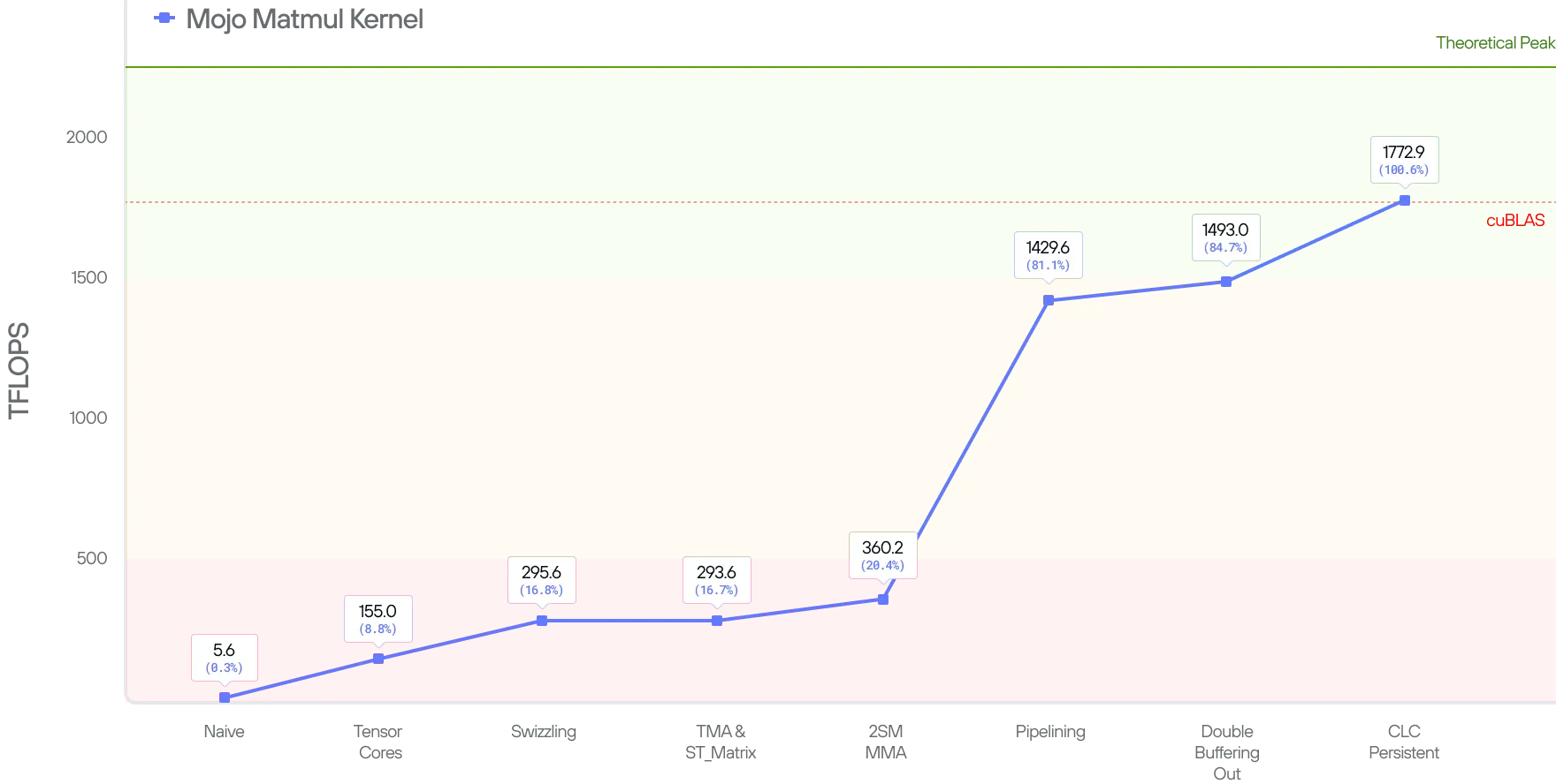
In this blog post, we’ll continue our journey to build a state-of-the-art (SOTA) matmul kernel on NVIDIA Blackwell by exploring the cluster launch control (CLC) optimization. At the end of the post we’ll improve our performance by another 15% and achieve 1772 TFLOPs, exceeding that of the current SOTA.

‍

Kernel 8 : CLC Persistent Kernel

In the part 3 post, we mentioned that the matmul kernel still suffers from 2 major overhead costs:

1. Shared memory and barriers initialization needs to restart between Waves (we will discuss what this means).
2. The writes to the C matrix don’t overlap.

In this section, we’ll discuss how we removed these two overheads using a persistent kernel.

What is a persistent kernel?

To understand persistent kernels, we must first explain what a wave is. In a GPU, a wave refers to a batch of thread blocks that can be assigned to all available streaming multiprocessors (SMs) at once. Kernel execution can be viewed as a sequence of waves processed one after another until all work is complete.

In the case of matmul—where thread blocks represent the entire workload and the thread block IDs corresponding to block tile coordinates—a persistent kernel means that the kernel author, rather than the hardware, controls the scheduling of these block tile coordinates.

In Hopper architecture, we can define a tile scheduler that works like this:

• Launch as many Cooperative Thread Arrays (CTAs) as you have available SM’s
• Make each one compute the matrix multiply accumulate (MMA) and store an output tile
• Once the write-out is complete, give it the coordinates of the next tile to compute
• Keep going for Num_Tiles / Num_SM’s iterations

The following code shows how we can fetches the next work tile to current CTA.

With the above we can show the high level code structure using a tile scheduler:

The scheduler keeps the CTA persistent by feeding it with new work tiles until there is no more work i.e. work_info becomes invalid. By keeping the CTA resident on the SM, we can eliminate the overhead time taken to launch the next block, and get our scheduling to look like this:

However, the static persistent kernel has a few issues:

1. It assumes that the kernel is always utilizing all SMs. This is not true if the GPU is launching multiple kernel at the same time.
2. It does not know which SMs are idle/busy.

These factors can cause sub-optimal scheduling if other kernels are running on the same GPU. It can also cause starvation on SMs if thread blocks go a few waves ahead. Both of these issues have been addressed in Blackwell using Cluster Launch Control (CLC).

A deep dive into the CLC scheduler

New in NVIDIA’s Blackwell architecture is a scheduler on the silicon. Rather than relying on software-managed distribution, the hardware now orchestrates work through an elegant producer-consumer model. The idea now becomes:

1. Launch as many thread blocks as the problem shape requires.
2. Scheduler warp (warp 4 of the 1st CTA in a cluster) tries to “cancel” work tiles by assigning them to idle SMs.
3. Scheduler warp also writes the coordinates to a dedicated shared memory location in all CTAs within the cluster, signaling the arrival of 16 bytes of data.
4. Once the signal arrives, all CTAs within the cluster read the coordinate from the shared memory location.

This process continues until all thread blocks are processed by the GPU.

A high level implementation of the tile scheduler looks like this in Mojo:

Here we use empty_mbar and full_mbar to signal when work tile coordinates arrive and are fetched. Looking closely, you can see that we also implemented pipelining for the TileScheduler. We'll discuss the rationale behind this design decision in the next section.

With this implementation, we can at least overlap the next wave’s Tensor Memory Accelerator (TMA) load with the current wave’s C write-out. But we still have more work to do to remove the overhead from CLC scheduling and the stalls between MMAs from different waves.

Pipelining CLC fetches

To remove the CLC scheduling overhead, we pipeline them. This is the same idea as prior kernels:

In the above code, if we assume a 2-stage pipeline then we reserve 2 shared memory locations for the CLC response for each CTA. The load_warp will always wait for the coordinate to be written into shared memory of the current pipeline state index, but the scheduler_warp can always race ahead and write the next coordinate in the next shared memory location.

The only scenario where the scheduler_warp needs to wait for the load_warp is when the pipeline index has looped through the entire pipeline and the coordinate still has not been fetched by the load_warp .

Now the scheduling looks better. It moves the overhead of scheduling the work tile to overlap with the next wave’s TMA load.

TMEM as a circular buffer

Using a single Tensor Memory (TMEM) address for accumulator introduces 2 major drawbacks:

• Idle Warps: While epilogue warps transfer data from TMEM → SMEM → GMEM, the producer and consumer warps sit idle. If they do work on the next tile, they’ll overwrite the data in tensor memory that the epilogue warps are reading from.
• Sequential MMA and output: The output and the next wave's MMA are still being executed sequentially. This is because of the data dependency from TMEM between the MMA warp and the output warp.

To resolve this, we can treat TMEM as a circular buffer just like what we did with shared memory for A and B. Let’s say we choose MMA_N == 256. Then, while epilogue warps write out results from columns 0-255, the mma warps could concurrently be accumulating the next tile's results in columns 256-511.

Conceptually, this is a natural optimization. We just need to define accum_full and accum_empty barriers to signal which stage of the TMEM buffer is empty or full. And because it only impacts our mma and epilogue warps, the code change to support this is minimal:

MMA warp

Output warp

After fixing the 2 major overheads mentioned above, we now have our optimal scheduling.

Comparing this to our Hopper (H100) matmul scheduling, we can see that every stage of the Blackwell (B200) kernel executes asynchronously. This is all thanks to Blackwell’s new tensor memory and CLC enabling a producer-consumer model to schedule work tile.

With all these optimizations in place, our kernel performs at 100.6% of cuBLAS at 1772.9 TFLOPs for shape 4096x4096x4096.

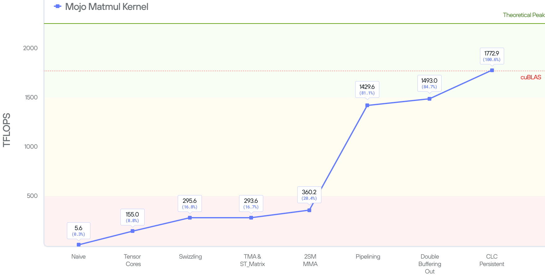
However, if we look at other shapes (such as 8192x8192x8192) then our performance is still at 90% of cuBLAS. So there are further optimizations we can make here.

Kernel 9 : Thread Block Swizzle

Now that we can schedule work tile to SMs, the only optimization remaining is to improve L2 cache hit. We can do this with a trick called block swizzling.

To understand this, we first need to visualize how CLC schedules block tiles to each wave. In the following plot let’s assume we are launching a 6x5 cluster—creating a 28 cluster-wise work tile.

Let’s also assume the GPU has 9 SMs available in each wave. The work tiles that are assigned to each wave is shown below.

Looking at Wave 0, we see that for matrix A, we need work tile ([0, 5], k) and for matrix B we need ([0, 1], k). That’s 6 loads for matrix A and 2 loads for matrix B from global memory. That’s because only work tile ([0, 2], k) from matrix A and ([0, 1], k) from matrix B can be reused for multiple work tiles. As a result, the memory tile can be evicted from L2 because of this low reuse rate.

The swizzling pattern allows us to move across the N dimension and create a zig-zag pattern, which help to schedule a batch of work tiles that share the same work coordinate. The number of tiles to move across the N dimension is called the block_swizzle_size . The optimal block_swizzle_size depends on the problem shape and the number of cluster-wise block tile being launched.

Now let’s look at an example of using block_swizzle_size of 2. We are now moving across the N dimension by 2 before moving down along the M dimension:

‍

Mapping this back to each wave, the work tiles that are scheduled to wave 0 and 1 now look like this:

‍

As you can see in wave 0, matrix A needs work tile ([0, 4], k) and matrix B needs work tile ([0, 1], k) from global memory. That removes one load from global memory compared to the scheduling without thread block swizzle.

Putting things together

In this blog post series, we’ve explained how we implemented increasingly optimized matmul kernels using features on the Blackwell GPU. The following table provides a recap of our kernel implementation and optimizations so far.

As you can see in wave 0, matrix A needs work tile ([0, 4], k) and matrix B needs work tile ([0, 1], k) from global memory. That removes one load from global memory compared to the scheduling without thread block swizzle.

Applying to Shapes in Production

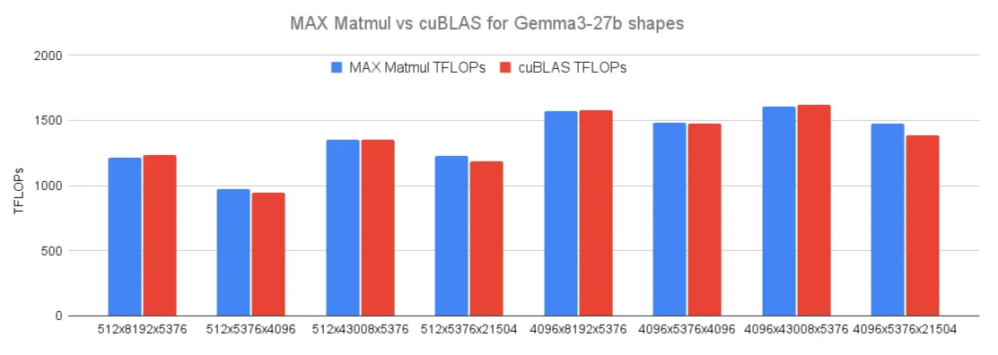
Up to now, and to make things simple, we have concentrated on square matrices with shapes such as 4096 and 8192. This is great for the purposes of the blog post, but these shapes do not occur in production LLMs. In paractice, the M dimension depends on the batch size and prompt lengths which ranges from O(10^2) to Q(10^3) instance. The N and K dimension correspond to the model. The figure bellow shows the shapes for the gemma-3-27B-it model.

When optimizing for shapes used in production, the key is to choose the optimal parameters including MMA shape, pipeline stages, block swizzling patterns, etc., to efficiently orchestrate the optimizations covered thus far. These parameters are chosen to minimize the workload per SM or equivalently maximize the use of all SMs. For instance, serving Gemma 3 involves a matmul of shape MxNxK = 512x8192x5376. Using 2xSM MMA instruction shape 256x256 we demonstrated before creates 512/128 x 8192/256 = 128 CTAs. Whereas, if we reduce the instruction shape to 256x224, the kernel creates 148 CTAs which perfectly maps to the 148 SMs on B200.

However, some shapes require nuance parameter choices which are hard to compute empirically, since there is a subtle trade-off between pipeline stages and output tiles (see part 3 of the series). The good thing is that Mojo has a builtin autotuning framework (kbench) to select the optimal parameters given a problem shape. Via autotuning, and using real workloads, MAX matches exceed the SOTA implementation by up to 6% when running Gemma 3 27B on NVIDIA Blackwell system.

‍

Summary

This blog post walked through how MAX outperforms SOTA implementations of matmul. Along the way, we showcased how the GPU hardware has become more complex with many features required to work in unison to achieve peak TFLOPs. As we look into the future, GPUs will become even more powerful and sophisticated. In turn, the programming patterns required to achieve peak performance must also become more sophisticated, and Mojo is up to the challenge.

We’ve shown how to program several GPU features directly in Mojo, but this is just the a taste. In subsequent blog posts, we’ll showcase the tools that help us write high performance code, describe how Mojo can achieve performance while retaining strong programming ergonomics, and discuss how you can use those patterns to also make your code portable across hardware. Stay tuned!