
A matrix is a rectangular collection of row vectors and column vectors that defines linear transformation. A matrix however, is not implemented as a rectangular grid of numbers in computer memory, we store them as a large array of elements in contiguous memory.
In this blog post, we’ll use Mojo🔥 to take a closer look at how matrices are stored in memory and we’ll answer the questions: What is row-major and column-major ordering? What makes them different? Why do some languages and libraries prefer column-major order and others row-major order? What implication ordering in memory have on performance?
Row-major order vs. column major order
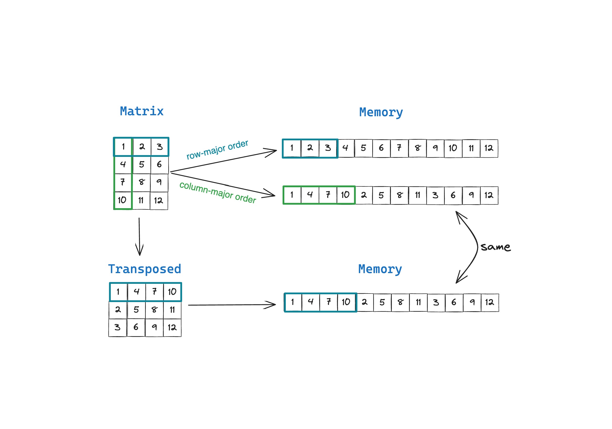
Row-major and column major are different approaches for storing matrices (and higher order tensors) in memory. In row-major order, row-vectors or elements in a row are stored in contiguous memory locations. And in column-major order, column-vectors or elements in a column are stored in contiguous memory locations. Since it’s faster to read and write data that’s stored in contiguous memory, algorithms that need to frequently access elements in rows run faster on row-major order matrices, and algorithms that need to frequently access elements in columns run faster on column-major order matrices.

Programming languages like MATLAB, Fortran, Julia and R store matrices in column-major order by default since they are commonly used for processing column-vectors in tabular data sets. The popular Python library Pandas also uses column-major memory layout for storing DataFrames. On the other hand, general purpose languages like C, C++, Java and Python libraries like NumPy prefer row-major memory layout by default.
Let's take an example of a common operation in data science, that involves performing reduction operations (sum, average, variance) on a smaller subset of columns in large tabular datasets stored in databases. Reduction operations on columns using column-major order matrices significantly outperform row-major order matrices since reading column values from contiguous memory is faster than reading them with strides (hops across memory). In the red box below, you can see the performance difference on my M2 MacBook Pro using Mojo. In the purple box, you can see that Mojo also outperforms NumPy in both NumPy’s row-major order and column-major order matrices.

Implementing row-major order and column-major order matrices in Mojo
To better understand how matrices are stored in memory, and how it affects performance let’s:
- Implement a custom matrix data structure in Mojo called MojoMatrix that lets you instantiate matrices with data in either row-major or column-major order
- Inspect row-major and column-major matrices and their memory layouts, and how they are related to each other and to their transposes
- Implement fast vectorized column-wise reduction operations for both row-major and column-major matrices and compare their performance.
- Compare their performance with NumPy’s row-major ndarrays (default, C order) and NumPy’s column-major ndarrays (F order)
It’s important to note that the order in which elements of a matrix are stored in memory doesn’t affect what the matrix looks and behaves like, mathematically. The row-/column- majorness is purely an implementation detail, but it does affect the performance of algorithms that operate on matrices. In the accompanying row_col_matrix.mojo file on GitHub, I’ve implemented a matrix data structure called MojoMatrix. MojoMatrix is a barebones matrix data structure that implements the following functions, which we’ll use to inspect and learn about the data layouts and its effect on performance.
- to_colmajor(): A function that accepts a MojoMatrix with elements in row-major order and returns a MojoMatrix with elements in column-major order
- mean(): A function that computes column-wise mean, in a fast, vectorized way that is 4x faster than NumPy’s ndarray.mean() when using NumPy’s column-major order or 25x faster than NumPy’s default row-major ordering.
- transpose(): A function that computes a vectorized transpose of a matrix, that we’ll use to inspect the elements in memory
- print() and print_linear(): A print function to print the matrix in matrix format, and a print_linear function that prints the elements of the matrix as they’re laid out in memory
- from_numpy(): A convenience static function that copies a NumPy array to MojoMatrix so we can measure performance and compare performance on the same data
- to_numpy(): A convenience function that copies MojoMatrix data to NumPy array to verify accuracy of operations performed in Mojo and NumPy
Let’s take a closer look at using MojoMatrix before we run benchmarks.
In this example we create a simple matrix that resembles the one displayed in illustration earlier in the blog post.
If you take a closer look, you’ll see that the matrix output says Row Major and you can verify from the output of print_linear() resembles the row-major order layout in the illustration earlier.
Now let’s convert our row-major order matrix to column-major order matrix using to_colmajor()
Notice that the output of print(M) is exactly the same as with the row-major order matrix. This is because how the matrix is stored in memory is an implementation detail, and does not and should not affect how you use the matrix.
You’ll also notice that the output of print_linear() is actually different. The elements have been re-ordered such that the columns of the 4x3 matrix are next to each other in memory.
How is matrix transpose related to row-major order and column-major order?
A transpose operation switches the rows and columns of a matrix without changing its contents.
If you have a matrix $M_{mxn}$ and you transpose it, then you get $M^{T}_{nxm}$ i.e. the rows and columns switched.

In the above figure, you can see that the order of elements of the transposed matrix $M^T$ in row-major order is exactly the same as the order of elements of the matrix is stored in column-major order. The key difference is that a transposed matrix $M^{T}_{nxm}$ has different properties mathematically, with the fundamental row and column spaces swapped, whereas storing the same matrix $M_{mxn}$ in column-major order is merely an implementation detail. We can implement this and compare the results using MojoMatrix and its transpose() and to_colmajor() functions
If you inspect the transpose() and to_colmajor() function implementation you will see that the only difference between these two is the dimensions $mxn$ vs $nxm$ and the actual reordering of elements is tucked away in an internal function called _transpose_order() that is shared by both.
How does row-major order vs. column-major order affect performance?
Now that we’ve built some intuition around row-major and column-major ordering, let’s discuss why it matters for performance. In data science, data scientists routinely load tabular data sets from databases or other sources and load them into Pandas DataFrame or NumPy’s ndarray and run operations such as averages, sums, medians or fit histograms on the columns of the datasets to better understand the data distribution. These data sets have certain properties:
- They are matrices that are “narrow and tall”, i.e. their number of rows far exceeds the number of columns
- Not every column or feature or attributes are useful, and many are discarded or ignored in computation
This means most of the data access pattern will be accessing all rows of specific columns that are not next to each other. Libraries like Pandas and programming languages like MATLAB, Fortran and R designed for statistical and linear algebra computations that have to deal with this type of data and data access pattern, are column-major order by default. Therefore it makes sense to have elements in a column be in contiguous memory ala column-major order.
To simulate this problem, let’s define a problem statement: On a 10000x10000 element matrix of double precision values, perform a mean() reduction operation on a subset of 1000 randomly selected columns. This ensures that most columns are not neighbors of each other.
NumPy benchmarking: row-major order vs. column-major order matrices
First, let’s benchmark a NumPy implementation to analyze the effect of row-major vs. column-major ordering. You can find the the accompanying file python_mean_bench.py on GitHub. In this benchmark we show two things:
- Find the average of all the columns in the 10000x10000 matrix
- Find the average of a subset of 1000 randomly selected columns
NumPy allows you to switch from the default C-style ordering (row-major order) to Fortran F-style ordering (column-major order) using the function np.asfortranarray() and you can see the big performance difference.
The first result is for calculating the average of every column, and you’ll see that the performance for row-major order and column-major order is small. Why isn’t there a much larger difference in performance? After all, accessing columns in a row-major order matrix requires strided memory access which know is slower.
NumPy implementation exploits the fact that the row values are still contiguous in memory and is able to reduce multiple columns at the same time using SIMD instructions. But this optimization won’t help us when the columns are randomly selected. Which is why you see the big performance difference in the second result: Mean of 1000 random columns, time (ms) where NumPy’s column-major order matrix is about 6x faster than NumPy’s row-major order matrix.
Mojo benchmarking: row-major order vs. column-major order matrices
Now let’s solve this task using MojoMatrix in Mojo. I won't get into the implementation details of MojoMatrix in this blog post, you can find the full implementation on GitHub. Here is the skeleton of the struct:
In the mean() function in MojoMatrix I’ve implemented a fast, vectorized reduction operation that works on both row-major order and column-major order matrices.
In the code above, I have two separate approaches for row-major and column-major order matrices.
Row-major order algorithm: In row-major order the column-vector values are not stored in contiguous memory, but are separated by a stride length = number of columns. We can still perform vectorized reduction by loading the system's SIMD width values using the function simd_strided_load[simd_width](offset=number_of_column). If the number of rows in the matrix is not a multiple of the system’s SIMD width, the spillover values are reduced in the second loop for idx_row in range(simd_multiple, self.rows) in a non-vectorized way.
Column-major order algorithm: In column-major order, the column-vectors are stored in contiguous memory locations, so loading values and reducing them using SIMD vectorization is much faster. Like before, we if the number of rows in the matrix is not a multiple of the system’s SIMD width, the spillover values are reduced in the second loop for idx_row in range(simd_multiple, self.rows) in a non-vectorized way.
In both cases, we verify that the results match the results in NumPy within a very small tolerance value. Here are the 🥁drum roll 🥁results:
In Mojo, the performance difference between row-major order and column-major order is significant. Column-major order delivers a 21x speedup over row-major order, for this problem. The entire implementation is 25 lines of Mojo code and it is 26x times faster than NumPy’s default row-major order implementation and 4x faster than NumPy’s column-major order implementation, both of which we saw in the previous section. All performance was measured on my MacBook Pro with M2 processor.
Conclusion
I hope you enjoyed this primer on row-major order and column-major order matrices, and why it matters for performance. If you’d like to continue exploring, here’s your homework:
- Try implementing matrix-vector product M@v using the implementation I shared as a starting point and benchmark the performance between row-major order M and column-major order M. (Hint: row-major order M should be faster, but why?)
- Try scaling transformations of columns on row-major order and column-major order matrices
- Implement matrix factorizations operations on row-major order and column-major order matrices.
There are a lot of benefits to using both, and it’s nice to have the option to switch between the two. Mojo makes it very convenient to express scientific ideas, without sacrificing performance. All the code shared in this blog post is on GitHub. Here are some additional resources to get started.
- Get started with downloading Mojo
- Head over to the docs to read the programming manual and learn about APIs
- Explore the examples on GitHub
- Join our Discord community
- Contribute to discussions on the Mojo GitHub
- Read and subscribe to Modverse Newsletter
- Read Mojo blog posts, watch developer videos and past live streams
- Report feedback, including issues on our GitHub tracker
Until next time🔥!