Today’s AI infrastructure is difficult to evaluate - so many converge on simple and quantifiable metrics like QPS, Latency and Throughput. This is one reason why today’s AI industry is rife with bespoke tools that provide high performance on benchmarks but have significant usability challenges in real-world AI deployment scenarios. This blog post focuses on support for dynamic shapes, a lesser-known but critical feature of AI infrastructure that significantly impacts real-world performance and usability. Full support for dynamic shapes is a technical feat the Modular team had to overcome, but we show that having it allows the Modular AI Engine to provide both the best in usability and the best in performance together (without compromising on either) in a single “it just works” package.
Modular's AI Engine is 5x faster on compile time and 2x faster at runtime, with full dynamic shapes support, when running BERT on the Glue dataset than other statically shaped compilers like XLA on Intel CPUs. It supports any model from popular frameworks, and our incredible performance extends to other datasets and models as well.
With the Modular AI Engine, AI developers get the best of both worlds: Our infrastructure combines the dynamic shapes support of PyTorch eager, TensorFlow Graphs, and PyTorch 2, with even better performance than XLA.

Dynamic input shapes in NLP models
Let’s define what dynamic shapes are by describing them in the context of a real-world use case. Natural Language Processing (NLP) is one of the most popular model families, used for everything from sentiment analysis to auto-completion, chat bots, LLMs, and much more.

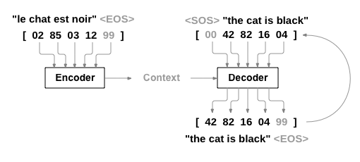
In most cases, NLP models take a text input (e.g., your question or statement to a chatbot) and produce outputs depending on the target task (e.g., an answer to your query). The input can range anywhere from short sentences of a few words to paragraphs of text content which are then turned into a “token stream” that roughly correspond to words. Each input has a different length known as a “sequence length”: for example, an input of “Modular supports dynamic shapes” often has a sequence length of 4. As you can imagine, if you were using a language translation model, you would commonly input sequences of varying lengths.

In an AI model, data is represented using tensors, and the varying sequence lengths means AI model execution needs to support what are known as “dynamic tensor shapes.”
Some production models are even more complex — they vary both in sequence length and also may have different batch sizes depending on incoming traffic volume. In other words, these tensor shapes vary across multiple dimensions. This scenario is significantly more complex, so we’ll save that topic for a future blog post and only consider inputs that vary on a single shape dimension in the rest of this one.
The increasingly important role of compilers in AI systems
If you are an experienced AI developer but you’ve never heard of dynamic shapes before, you’ve likely been deploying models into production via dynamic infrastructure like PyTorch eager, PyTorch’s default execution mode.
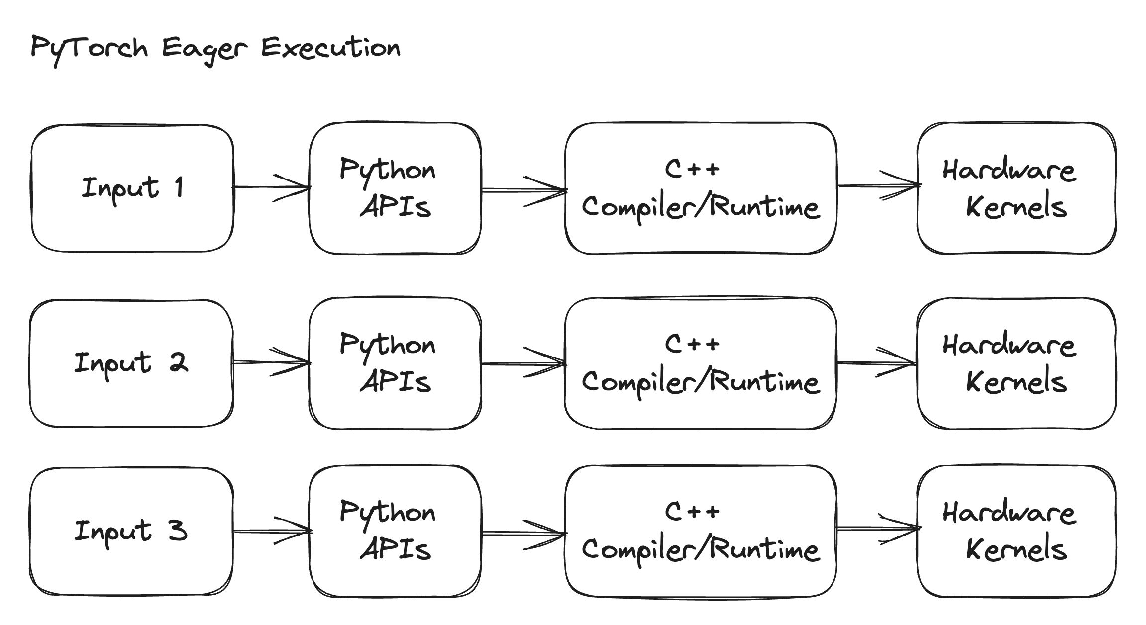
As we discussed in our launch video, modern AI frameworks comprise three layers — a thin Python API, C++ systems code, and hardware kernels (C++ or CUDA). PyTorch’s eager execution mode executes operators in a model as they are encountered, round-tripping through the whole stack, from Python APIs down to the hardware kernels, and returns a final result. The same pattern happens on each new input, meaning that eager execution supports dynamic shapes by design. Eager execution in PyTorch saves you from having to think about your input shapes in your development workflow.

However, there are a couple of problems with “op-by-op” eager dispatch:
- Eager execution doesn’t maximize performance because it doesn’t take a holistic view of the program, instead executing the model one operation at a time (also roundtripping through slow Python code).
- It doesn’t generalize and scale well to support many diverse hardware backends for reasons we described in a previous blog post.
- Finally, for production deployment, server OS environments may not provision Python runtimes or dependencies, making models harder to deploy in frameworks with eager mode on these systems.
For these reasons, plus the increasing need to support larger and more complex models like LLMs, the AI industry is moving toward compiler-based approaches.
The traditional compiler approach to supporting dynamic shapes
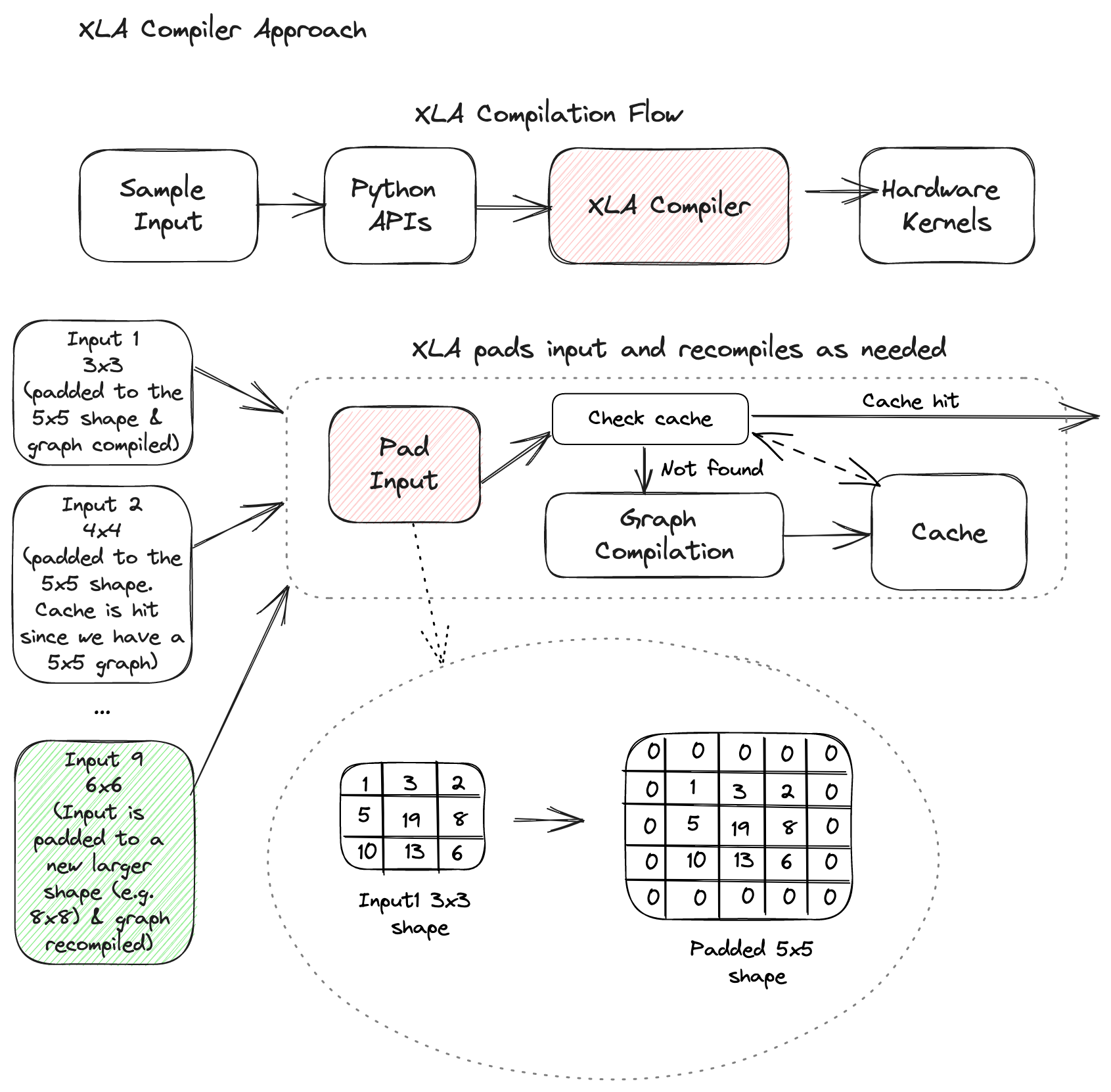
Compilers like clang and gcc are widely used for traditional programming, but compilers in AI are limited to more exotic use cases. While early attempts at AI compilers like XLA (which is used by Google’s TensorFlow and JAX frameworks) and Glow (which was developed at Meta) show impressive performance wins, they don’t support dynamic shapes, forcing complexity onto the deployment engineer before they can use these tools.
Use of XLA and Glow requires that the user statically compile a graph for each specific sequence length. A common approach is to compile for the longest expected sequence length (generally via providing a sample input into the compilation process), cache the compiled graph in memory, and reuse it for all incoming inputs. Any inputs that are shorter than the longest expected sequence length are appended with 0’s (”padded”) to make them valid inputs into the compiled graph.

The problems with padding queries to a longer sequence length are threefold:
- It slows the performance of short queries to that of the longest sequence. Your performance for shorter sequence lengths (e.g., a sequence length 4), should be meaningfully better than that of your max sequence length (e.g., sequence length 128), but that won’t happen when you work around lack of dynamic shapes with padding. Practically, this means higher latency and lower resource efficiency, and higher costs to support the same set of inputs.
- If any input is larger than the largest expected static sequence length, the model must be recompiled to support the input. This recompilation happens at runtime, so compile time directly impacts user experience and long tail latency. This paradigm is untenable to most production scenarios when compilation can take minutes or even hours, so these queries typically just fail.
- Each compiled version contributes to a larger binary size, which increases memory footprint, impacting cost and potentially impacting the viability of a model on resource-constrained devices.
Other hybrid approaches that have been tried
While we have primarily described two extremes — Eager execution (PyTorch) and static compilers (XLA) — different hybrid approaches exist. A few of note are PyTorch-XLA execution, TensorFlow graph execution, and PyTorch 2 graph execution.
Torch-XLA adds a JIT compiler to PyTorch eager. In other words, execution is the same as we described early, but it leverages XLA to compile groupings of operations on the fly. In doing so, it uses recompilation and “graph breaks” to address the static limitations of XLA. However, this approach can also not reach peak performance as it isn’t compiling across the whole program and incurs the overhead of XLA compile times during runtime.
TensorFlow graph execution is the most commonly used infrastructure in production today. It is, by definition, a compiler — users capture a graph via tracing using the TF2 tf.function API (or build a graph directly in TF1). That graph is dynamically compiled and executed via the TF engine and C++/CUDA kernel libraries. The Modular AI has significantly better performance than TensorFlow graph execution, despite TensorFlow also supporting dynamic shapes, as we describe in more detail below and on our performance dashboard.
More recently, PyTorch 2 has provided a graph programming paradigm via their torch.compile() API. This graph mode provides dynamic shape support for all the reasons we mentioned above, but it's not on by default. These features are still in beta in PyTorch 2 and are sparsely used in production.
The benefits of Modular’s dynamic compiler for AI developers
To demonstrate the benefits of dynamic shape support in the Modular AI Engine, we can compare it to existing infrastructure on a real-world dynamic use case.
We leverage BERT-base, a popular transformer-based language model from HuggingFace, and compare Modular to TensorFlow graph execution using the SavedModel format (tf.saved_model.load() APIs). Both TensorFlow and the JAX framework can use the XLA optimizing compiler, e.g. by using an additional argument: tf.function(jitcompile=true). XLA does not support dynamic tensor shapes. We will not benchmark against PyTorch 2 given its limited usage in production today, but will discuss it in more detail in a future blog post.
We fine-tuned our model on the GLUE benchmark’s CoLA dataset, which consists of a set of grammatically correct English sentences drawn from published linguistics literature. The goal of the model is to test the grammatical acceptability of a given sentence. We measure the compilation time that each framework takes to process the input tensor and execution time (or “inference time”). We report the total execution time by summing the run times for all the input tensors that were processed by the framework. Finally, we also double-checked the accuracy of all the three frameworks to ensure consistent results on the various CPU platforms we tested on.
All results were gathered on CPU platforms available in the cloud today - Intel Skylake (c5.4xlarge on EC2), AMD EPYC (c5a.4xlarge on EC2) and AWS Graviton2 (c6g.4xlarge on EC2).
Naive execution of each sequence
In this first experiment, we make no attempt to pad the input tensors — each unpadded tensor is run iteratively through all the three frameworks and we measure the compilation time and execution time for each input.
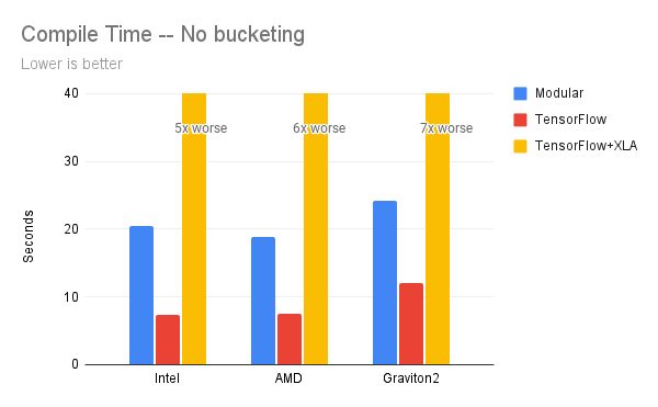
On compilation time, the Modular AI Engine is 5x-7x faster than the compilation times of XLA on the various CPU platforms. Since TensorFlow (tf.function) compiles the graph at the first invocation of the model (i.e. just-in-time), we run random data for a few iterations before measuring the execution time for TensorFlow. The TensorFlow “compilation time” in the chart below refers to the time taken for TensorFlow to load the model and initialize the appropriate APIs to load the graph.
The Modular AI Engine compiles the graph, and the result supports dynamic input tensors - we can see the Modular AI Engine can execute models faster than each variant of TensorFlow out-of-the-box. On the three CPU platforms, the XLA compilation times are an order of magnitude worse compared to Modular. For better readability, the XLA compilation times are cropped on the chart.

On the three CPU platforms, the Modular AI Engine delivers speedups of 3x-9x vs default TensorFlow on BERT, a very commonly optimized language model. XLA requires much longer compile time than TensorFlow but does deliver better execution performance. However, the Modular AI Engine still delivers 2x-4x faster better performance than XLA.

Mitigation using bucketing and padding strategies
Since the input tensor shapes can be quite dynamic depending on the dataset, one mitigation strategy that is frequently employed in real-world scenarios is to reduce the variance across shapes via bucketing. This strategy typically involves creating multiple model instances that support a range of input shapes and then padding the input tensors up to the maximum size in the closest sub-range. The bucketing strategy itself may be tricky - as choosing too large a number of sub-ranges will cause many recompilations and choosing too few will cause extra padding on the tensors and thus, unnecessary compute cycles. Moreover, having to scale multiple model instances based on incoming traffic volume and relative distribution of input shapes can be quite tricky. This mitigation strategy is only required for compilers which don’t support dynamic shapes - as the Modular AI Engine is fully dynamic, users don’t need to worry about it!

To show the impact of this mitigation strategy on our data, we test the performance XLA with bucketing, repeating the experiments described earlier in the section. More specifically, we pick four sub-ranges for the input sequence lengths: 8, 16, 32 and 64 (powers of 2) and pad the input tensors to the maximum length of each sub-range.
With the bucketization strategy, XLA’s compile time reduces significantly as it is only compiled once for each bucket, bringing it closer to Modular’s compile time on these CPU platforms.

However, even with this strategy, the Modular AI Engine is still 2x-4x faster on model execution time compared to TensorFlow+XLA (and using the same numerics of course) on various platforms.

Sign up to start using the AI Engine now!
Full support for dynamic shapes is just one of the many ways the Modular AI Engine simplifies your life while reducing your cost and latency. You get the benefit of state of the art compiler and runtime technology, without being forced to work around capability limitations or having to juggle many “point solution” tools that help accelerate an individual model or architecture.
You can get started today with the Modular AI Engine by signing up here and explore the APIs in our documentation portal.


