We started this blog post series to describe how to write Mojo🔥 for the Mandelbrot set to achieve over 35,000x speedup over Python. To recap the optimizations so far, in part 1 we ported the code into Mojo to get around a 90x speedup, and then, in part 2 we vectorized and parallelized the code to get a 26,000x. This blog post continues this journey to show another performance technique that takes well beyond our promised 35,000x speedup goal.

‍

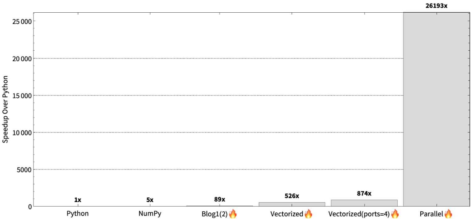
Recall that our parallelism strategy in the previous blog post is that each CPU core gets an equal number of rows to process. Pictorially, the idea is that we can evaluate each set of rows independently and achieve speedup proportional to the number of cores.

‍

Load imbalance

However, the animation in Figure 2 is deceiving. Partitioning the work so that each thread worker gets a set of rows is fine when the work is the same across the rows, but that’s not the case for the Mandelbrot set. Partitioning this way creates a load imbalance, since one pixel of the Mandelbrot set may finish after a single iteration and another pixel may use MAX_ITERS iterations. This means that the number of iterations per row is not equal, and therefore some threads will be sitting idle, because they finish the computation faster than other ones.

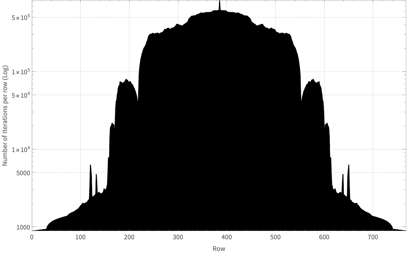
To demonstrate the imbalance, we plot the total number of iterations each row performs within the Mandelbrot set. As shown in the figure below, some rows require less than 1000 iterations before they escape whereas others require over 800,000 iterations. 

If you partition in a way that each thread gets a sequential number of rows, what happens is that all threads will wait until the middle set of rows finishes (assigned to some core) before completion. There are multiple ways to alleviate this, but the easiest way is to over-partition. So, instead of each thread getting a set of rows divided equally amongst the cores, we have a work-pool and create a work item for each row. The threads pick items from the thread pool in round-robin fashion.

Thankfully, Mojo includes a high-performance concurrent runtime, so we do not have to create a thread pool or do the round-robin picking and execution ourselves. Mojo’s runtime includes advanced features to fully utilize many-core systems like this one.

fn compute_row(y:Int):
    let cy = min_y + h * scale_y

    @parameter
    fn compute_vector[simd_width:Int](w:Int):
        let cx = min_x + iota[DType.float64, simd_width]() * scale_x
        output.simd_store[simd_width](Index(h,w), 
                mandelbrot_kernel(ComplexSIMD[DType.float64, 
                                              simd_width](cx,cy))

    vectorize[num_ports * simd_width, compute_vector](width)

with Runtime(num_cores()) as rt:
    let partition_factor = 16 # Is autotuned.
    parallelize[compute_row](rt, height, partition_factor * num_cores())
    

‍

We can evaluate the program as we over partition by 2, 4, 8, 16, and 32 factors. The results are shown below:

‍

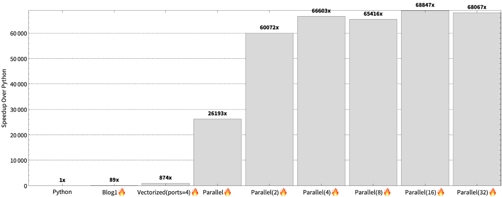
Effectively, we get a 2.3x speedup over the parallel version and 78x speedup over the vectorized implementation. An acute reader will ask whether it’s advantageous to partition even further – within a row. The answer is “maybe” if the row-size is large, but in our case it is 4096. Furthermore, within a row, pixels tend to be more correlated. This is advantageous for SIMD, since it means that work is not wasted within a vector lane. 

Why are we getting more than 35,000x speedup?

Why are we getting a 68,000x speedup instead of the advertised 35,000x speedup? In short, the benchmarking system is different. During launch, we evaluated on an AWS r7iz.metal-16xl 32-Core Intel Xeon Gold 6455B, but in this blog we evaluated on a GCP h3-standard-88 which uses an 88-Core Intel Xeon Platinum 8481C. The reason we do not use the r7iz.metal-16xl instance is because it is no longer available. But that said, we don’t mind exceeding expectations!

A higher core count and faster clock speed generally improve Mandelbrot problem speedup, and this actually shows the benefit of Mojo. Computers are only getting faster and bigger – core count is only going to increase and so (to a lesser extent) will the clock frequency. In general, you can expect speedup to double over the sequential version when you double your core count, while increasing your clock speed will exacerbate the significance of interpretation overhead. Additionally, such hardware scaling does not require Mojo code to be changed. In fact, we did not optimize the program across the instance types, but we are still able to get a performance improvement. 

Another question is why “we are getting a 2x speedup over the r7iz instance and not a 2.7x?” The answer is that the problem size is too small to saturate the CPUs and we did not optimize for the h3-standard-88 instance. For example, hyper threading is beneficial in general for the Mandelbrot computation, but we were unable to enable hyper threading on the h3-standard-88 instance type.

Performance recap

To summarize the optimization journey in the first 3 blog posts. In the first blog we first started by just taking our Python code and running it in Mojo, added some type annotations to the Mojo code, and performed algebraic simplifications. In the second blog post, we vectorizing the code, evolved that to utilize multiple ports, and then made the sequential implementation parallel to exercise all the cores on the system. Finally, in this blog post, we used oversubscription to resolve the load imbalance due to parallelism. During this journey we achieved 46x to 68,000x speedups over Python. As shown below.

‍

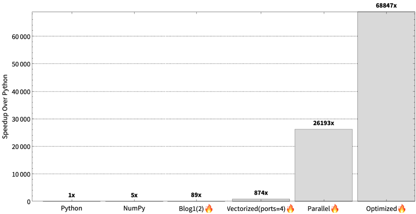
Again, it’s hard to read such massive speedups. So, to better show the differences in log scale:

‍

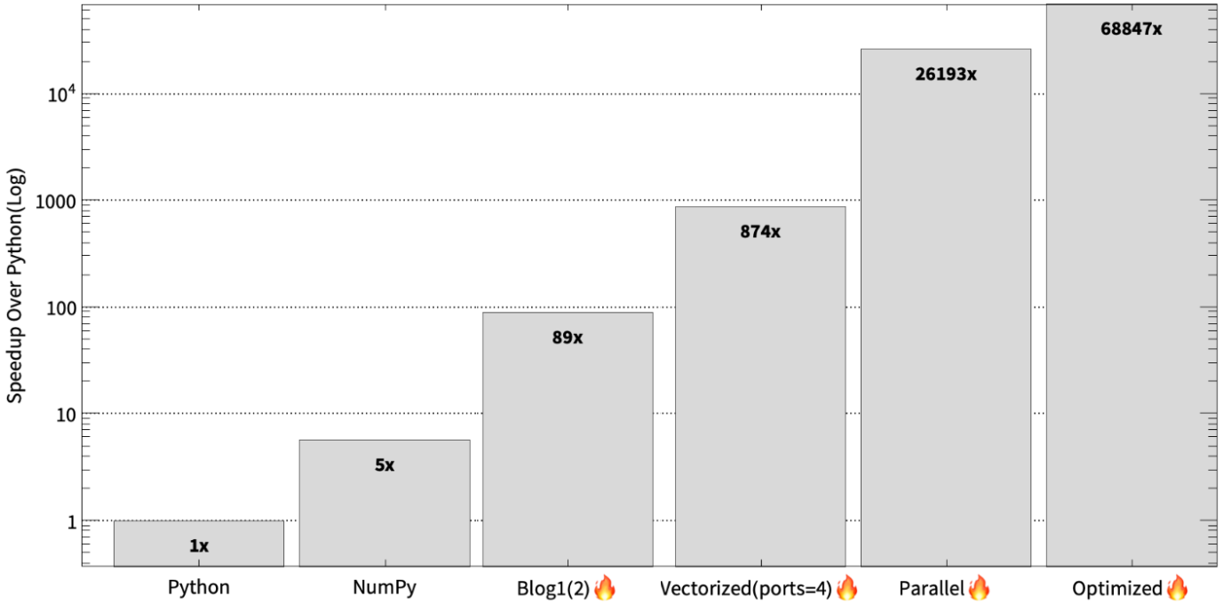
As shown below, our implementation achieves over 68,000x speedup over Python on this machine, and using oversubscription we are able to get 2x speedup over our previous parallel version.

Conclusion

In this blog post we explained the final optimization necessary to achieve the 35,000x claim made during launch. In the process, we accidentally overachieved and got a 68,000x speedup!

Throughout these blog posts, we showed that Mojo affords you great performance while being portable and easy to reason about. Performance does not come for free, however, and thus one has to be cognizant of the underlying hardware and algorithms to be able to achieve it. 

We employ the same principles when developing high performance numeric kernels for the Modular AI Engine. If you are interested in making algorithms fast and driving state-of-the-art AI infrastructure from the ground up, please consider joining Modular’s exceptional team by applying to our Kernel engineer role or other other roles available on our careers page.