Learning a new programming language is hard. You have to learn new syntax, keywords, and best practices, all of which can be frustrating when you’re just starting. In this blog post, I want to share a gentle introduction to Mojo from a Python programmer’s perspective. Rather than focus on the language details such as Mojo’s programming model and syntax, which you can find in the Mojo programming manual, I’ll focus on an example-driven introduction that will gently guide you to a land of Mojo familiarity. The example used in this blog post is available in the Mojo Playground, so if you haven’t already signed up for Mojo - do so now!

Mojo🔥: A familiar approach

Mojo should feel very familiar to any Python programmer, as it shares Python’s syntax. But there are a few important differences that you’ll see as we port a simple Python program to Mojo. The first thing you’ll notice is that Mojo really shines in the performance department. “But Python is no slouch – NumPy is really fast!” you might say, and you’d be right. However, if you look under the hood of NumPy’s elegant Python API, you’ll see that all the computationally intensive code is written in C/C++, which is where its performance comes from.

With Mojo, you can write high-level code like Python and leverage Mojo’s lower-level features to explicitly manage memory, add types, etc., to get the performance of C (or better!). This means you get the best of both worlds in Mojo and don’t have to write your algorithms in multiple languages.

Before we get started, here are a couple of housekeeping items:

• Mojo is still very early in its development phase and the language, and tooling aren’t ready to support the migration of large Python projects. We expect that Python users will initially port small, computationally demanding sections of their code to Mojo and then migrate more significant parts of their code base over time as the language and tooling mature. We are adding many new language features each week, and you should follow the regular Changelog to get updates.
• The Mojo Playground environment is not always stable. You will be able to reproduce the output results of the calculations but the performance (execution time) may vary, and you may not see the performance shown below. The goal of this blog post is to introduce you to Mojo, not to benchmark its performance.

From Python to Mojo: A simple example

Let’s start with a simple example that calculates the Euclidean distance between two vectors. This is mathematically expressed as the L2-norm of the difference vector $||\vec{a}-\vec{b}||$ where $\vec{a}$ and $\vec{b}$ are two n-dimensional vectors, and I’ll discuss the implementation details in the algorithm section below. Euclidean distance calculation is one of the most fundamental computations in scientific computing and machine learning, used in algorithms like k-nearest neighbors and similarity search. In this example, you’ll see how you can get faster-than-NumPy performance on this task, using high-dimensional vectors with Mojo. It’s a computationally intensive problem, so we’ll build a solution from scratch, starting with Python, and bring it over to Mojo to improve performance. 

My goal with this example is not to build the fastest program for this task, but to introduce Mojo and its syntax as a Python programmer. 

Where do I run this example? - The Mojo Playground

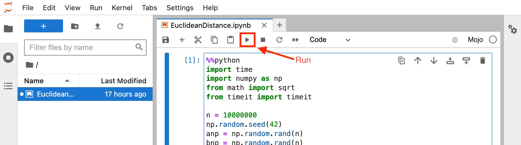
The code in this blog post can be copied and pasted into a new Jupyter notebook on Mojo Playground. First, head over to playground.modular.com to access or sign up to access Mojo on a hosted JupyterLab server. Once you have your playground open, create a new Notebook. Paste each code block in this blog post into a new Jupyter Notebook cell and press the Run button on the menu bar or hit Shift+Enter on your keyboard to run the cell and see the output. We're working to make the code in this blog post available as a Notebook in Mojo Playground soon!

‍

Algorithm implementation details

Calculating the Euclidean distance is fairly straightforward: 

1. Calculate the element-wise difference between two vectors to create a difference vector
2. Square each element in the difference vector
3. Sum up all the squared elements of the difference vector
4. Take the square root of the sum

These 4 steps are illustrated in the diagram below:

‍

In our implementation, the dimension of the vector n is the number of elements in our array or list. In pure Python, you’d write it down like this:

def python_naive_dist(a,b):
    s = 0.0
    n = len(a)
    for i in range(n):
        dist = a[i] - b[i]
        s += dist*dist
    return sqrt(s)

Euclidean distance in pure Python

First, let’s set a baseline by running and benchmarking pure Python performance for the Euclidean distance calculation. To verify the distance calculation is numerically accurate across Python and Mojo implementations, we’ll create two random NumPy arrays of 10 million elements each and re-use them throughout the example. For the pure Python implementation, we’ll convert these NumPy arrays into Python lists, so we only use data structure native to Python.

Mojo Playground tip: Add the %%python at the top of the Jupyter to instruct the Mojo Jupyter kernel to run this code as Python interpreted code and not as Mojo compiled code. 

First, let’s create 2 random vectors with 10,000,000 elements using the code below.

%%python
import time
import numpy as np
from math import sqrt
from timeit import timeit

n = 10000000
anp = np.random.rand(n)
bnp = np.random.rand(n)

alist = anp.tolist()
blist = bnp.tolist()

def print_formatter(string, value):
    print(f"{string}: {value:5.5f}")

‍

Now, we’re ready to calculate the Euclidean distance in pure Python.

%%python
# Pure Python iterative implementation
def python_naive_dist(a,b):
    s = 0.0
    n = len(a)
    for i in range(n):
        dist = a[i] - b[i]
        s += dist*dist
    return sqrt(s)

secs = timeit(lambda: python_naive_dist(alist,blist), number=5)/5
print("=== Pure Python Performance ===")
print_formatter("python_naive_dist value:", python_naive_dist(alist,blist))
print_formatter("python_naive_dist time (ms):", 1000*secs)

=== Pure Python Performance ===
python_naive_dist value:: 1290.91809
python_naive_dist time (ms):: 790.43060

‍

The pure Python implementation takes about ~790 ms to run. Take a note of the Euclidean distance value of 1290.91809, we’ll use that to verify that the subsequent implementations are numerically accurate.

Python + NumPy implementation

To be fair to Python, rarely do Python programmers use Python native data structures for machine learning and scientific computing. The de facto standard for such use cases is the NumPy package, which provides the n-dimensional array data structure and optimized functions that operate on them. Since we already created a random NumPy vector in the previous step, we’ll use the same numpy arrays and calculate the euclidean distance using NumPy’s vectorized numpy.linalg.norm function that computes the norm on the difference vector. We measure the execution time of the NumPy implementation below.

%%python
# Numpy's vectorized linalg.norm implementation 
def python_numpy_dist(a,b):
    return np.linalg.norm(a-b)

secs = timeit(lambda: python_numpy_dist(anp,bnp), number=5)/5
print("=== Python+NumPy Performance ===")
print_formatter("python_numpy_dist value:", python_numpy_dist(anp,bnp))
print_formatter("python_numpy_dist time (ms):", 1000*secs)

 === Python+NumPy Performance ===
python_numpy_dist value: 1290.91809
python_numpy_dist time (ms): 24.31807

‍

The time it took to calculate the Euclidean distance to the exact same value of 1290.91809 went from ~790 ms to ~24 ms: that’s about 30 times faster using NumPy’s faster C/C++ implementation under the hood.

Can we run it faster with Mojo? Let’s find out!

Our first Mojo implementation

Mojo offers Python’s usability with optional low-level control like C. Let’s start with a Python-like implementation in Mojo and see what performance we get. First, we need a data structure for our vectors. Mojo offers a Tensor data structure which allows us to work with n-dimensional arrays, and for this example we’ll create two 1-dimensional Tensors and copy over the NumPy array data to it.

from Tensor import Tensor
from DType import DType
from Range import range
from SIMD import SIMD
from Math import sqrt
from Time import now

let n: Int = 10_000_000
var a = Tensor[DType.float64](n)
var b = Tensor[DType.float64](n)

for i in range(n):
    a[i] = anp[i].to_float64()
    b[i] = bnp[i].to_float64()

‍

Let’s dissect this piece of Mojo code. First, you'll notice that we have new variable declarations let and var which may look odd at first glance since this is not familiar Python syntax. Mojo offers optional (except in some cases, more on that later) variable declarations to declare variables as immutable with let (i.e. cannot be modified after creation) or mutable with var (i.e. can be modified). There are two benefits to using variable declarations - type safety and performance. Second, you’ll also notice that the Tensor function has both square brackets and round brackets () with this format:

Function[parameters](arguments)

In Mojo "parameters" represent a compile-time value. In this example we’re telling the compiler, Tensor is a container for 64-bit floating point values. And arguments in Mojo represent runtime values, in this case we’re passing n=10000000 to Tensor’s constructor to instantiate a 1-dimensional array of 1 million values.

Finally, in the for-loop we assign numpy array values to Mojo Tensor. We’re now ready to calculate the Euclidean distance measure in Mojo.

‍Calculating the Euclidean distance in Mojo

Let’s bring our Python example over to Mojo and make a few changes to it. Below is our Mojo function for calculating Euclidean distance. Can you spot the few key differences vs. the Python function?

def mojo_naive_dist(a: Tensor[DType.float64], b: Tensor[DType.float64]) -> Float64:
    var s: Float64 = 0.0
    n = a.num_elements()
    for i in range(n):
        dist = a[i] - b[i]
        s += dist*dist
    return sqrt(s)

‍

Notice that this is very similar to our Python code, except that we’ve added types in the function arguments: a: Tensor[DType.float64], b: Tensor[DType.float64] and return type Float64. Unlike Python, Mojo is a compiled language and even though you can still use flexible types like in Python, Mojo lets you declare types so the compiler can optimize the code based on those types, and improve performance.

Here DType.float64 parameter of our Tensor specifies that it contains 64-bit floating point values. Float64 return type represents a Mojo SIMD type, which is a low-level scalar value on the machine register. We also declare the variable s with the var keyword which tells the Mojo compiler that s is a mutable variable of type Float64. Now we’re ready to benchmark our Mojo code.

let eval_begin = now()
let naive_dist = mojo_naive_dist(a, b)
let eval_end = now()

print_formatter("mojo_naive_dist value", naive_dist)
print_formatter("mojo_naive_dist time (ms)",Float64((eval_end - eval_begin)) / 1e6)

=== Mojo Performance with minimal code changes ===
mojo_naive_dist value: 1290.91809
mojo_naive_dist time (ms): 70.77003

‍

The execution time dropped down to ~70 ms from ~790 ms in pure Python, that’s about 11x faster. However, that is still slower than Python+NumPy’s ~40 ms but pretty good without having to re-write our function in C/C++. But we’re not done yet! We’re leaving a lot of performance on the table that we can recover with a few more minor code changes. Let’s see how.

Speeding up our Mojo🔥 code!

Just like in Python, def functions in Mojo are dynamic, flexible and types are optional which makes it easier to port Python functions to Mojo. However, there are a few key differences in how arguments are processed. In Python arguments to functions are references to objects and if modified, their changes are visible outside the function. In Mojo, def functions make a copy of all arguments and this introduces an overhead when dealing with large Tensors like we are. Therefore, to speed up our code further we need to:

1. Pass Tensor values by reference so no copies are made
2. Introduce strict typing and declare all variables 

Here’s our updated function that addressed both (1) and (2)

fn mojo_fn_dist(a: Tensor[DType.float64], b: Tensor[DType.float64]) -> Float64:
    var s: Float64 = 0.0
    let n = a.num_elements()
    for i in range(n):
        let dist = a[i] - b[i]
        s += dist*dist
    return sqrt(s)

‍

The first change you’ll notice is that the def has been replaced by fn. In Mojo, fn functions enforce strict type checking and variable declarations. The default behavior of fn is that arguments and return values must contain types and fn arguments are immutable variables. While def allows you to write more dynamic code, fn functions can improve performance by lowering overhead of figuring out data types at runtime and helps you avoid a variety of potential runtime errors. You can read more about the difference between fn and def in the Mojo programming manual.

Since all variables in fn functions have to be declared, we also declare n and dist with let and we’re ready to benchmark our updated code.

let eval_begin = now()
let naive_dist = mojo_fn_dist(a, b)
let eval_end = now()

print("=== Mojo Performance with fn, declarations and typing and ===")
print_formatter("mojo_fn_dist value", naive_dist)
print_formatter("mojo_fn_dist time (ms)",Float64((eval_end - eval_begin)) / 1e6)

=== Mojo Performance with fn, declarations and typing and ===
mojo_naive_dist value: 1290.91809
mojo_naive_dist time (ms): 13.82901

‍

Our Mojo code execution time dropped down to ~13 ms. That’s almost 2x faster than the NumPy which is implemented in C/C++ and 60x faster than the pure Python implementation. Let’s take a look at the Python and Mojo code side by side so you can appreciate how little you had to change the code to see the performance improvements.

Conclusion

There is a lot more to discuss about Mojo. For now, I hope you found this blog post to be a quick and gentle introduction to Mojo from a Python programmer’s perspective. There are more things to try to speed up our code, including better ways to allocate memory, vectorization, multi-core parallelization, and more.  explore these topics in upcoming blog posts. The full Jupyter notebook is available on Mojo Playground – head over to the Playground and run the example yourself! 

Now it’s your turn! How would you improve this code? Do you have ideas for other examples? We’d love to hear from you! Join our awesome community on Discord and share your Mojo journey with us on social media. Until next time 🔥!